pgmult: code for easy correlated multinomial models

The code in this repository implements the methods and models described in the paper Dependent multinomials made easy: stick-breaking with the Pólya-gamma augmentation. In particular, this package can be used for learning and inference in

• correlated topic models (CTMs) (in pgmult.lda),
• dynamic topic models (DTMs) (also in pgmult.lda),
• spatio-temporal count models with Gaussian processes (count GPs) (in pgmult.gp)
• linear dynamical system models for text (in pgmult.lds),
• or any new models you build using latent Gaussians and the stick-breaking logistic map to induce dependencies among multinomial or categorical parameters!

Example: fitting a correlated topic model

You can find pretty thorough code for fitting correlated topic models in experiments/ctm.py, which includes functions for downloading both the 20 Newsgroup dataset and the AP News dataset and comparing the performance of several inference methods. Here we'll just sketch the basic interface. We'll use several utility functions that can be found in experiments/ctm.py.

First, we load a dataset and split it into training and test data:

V=4000# a vocabulary of the 4000 most common wordstrain_frac=0.95# use 95% of the data for trainingtest_frac=0.5# on the test documents, hold out half of the wordsdata, words=load_ap_data(V)
train_data, test_data=split_test_train(data, train_frac=train_frac, test_frac=test_frac)

Next, we set some hyperparameters and instantiate a correlated topic model object (a.k.a. correlated Latent Dirichlet allocation, or LDA), passing in the training data:

frompgmult.ldaimportStickbreakingCorrelatedLDAT=50# 50 topicsalpha_beta=0.05# smaller alpha_beta means sparser topicsmodel=StickbreakingCorrelatedLDA(train_data, T, alpha_beta)

We're ready to run some inference! We can run iterations of a Gibbs sampler by calling the resample method of model. We'll just wrap that call in a function so that we can compute training likelihoods as we go:

defresample():
model.resample()
returnmodel.log_likelihood()
training_likes= [resample() for_inprogprint_xrange(100)]

Finally, we can plot the training likelihoods as a function of the iteration number

importmatplotlib.pyplotaspltplt.plot(training_likes)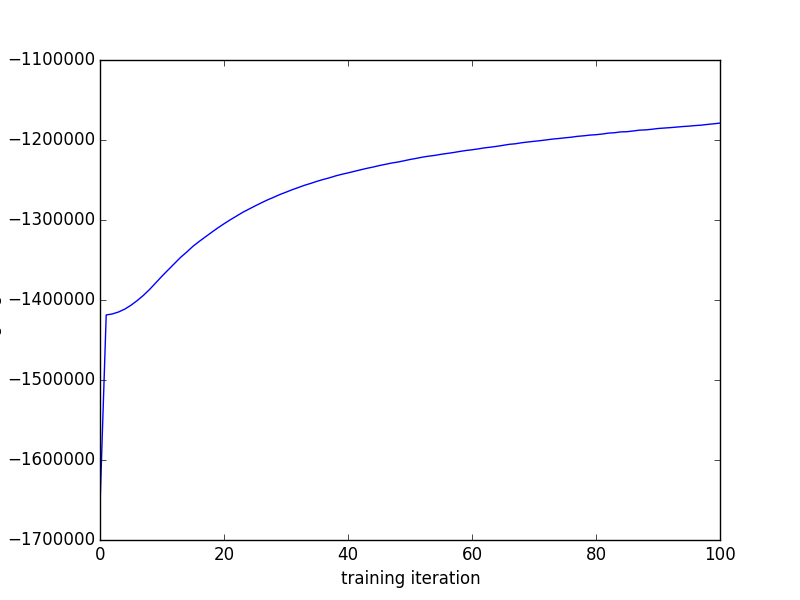

This Gibbs sampling algorithm is in some ways an improvement over the variational Expectation-Maximization (variational EM) algorithm used in the original CTM code because it's an unbiased MCMC algorithm, while the variational EM algorithm computes biased expectations in its E step. That means, for example, that you can compute unbiased estimates of arbitrary posterior or predictive expectations and drive the variance as low as you want, if you're into that kind of thing.

But the real point of this library isn't to provide fast MCMC algorithms for correlated topic models. The point of pgmult is to make constructing such algorithms much easier for all kinds of models.

Example: implementing a correlated topic model

The variational EM algorithm for CTMs isn't so easy to implement; just check out Appendix A of the CTM paper for the details on the variational E step. It's a block coordinate ascent procedure in which one block is optimized using nonlinear conjugate gradients and another is optimized with Newton's method subject to nonnegativity constraints. That's a powerful algorithm, but it does make deriving and implementing such algorithms for similar models look difficult, especially if you just want to embed a CTM in some other model.

The research behind pgmult is about developing an alternative inference strategy based on Pólya-gamma augmentations that yields algorithms which are both easy to derive and easy to implement. In fact, on top of a vanilla LDA implementation, which takes just a few dozen lines in pgmult.lda._LDABase, with pgmult the main inference step in a correlated topic model takes just a handful of lines.

Here we'll show the key lines in the implementation of StickbreakingCorrelatedLDA, leaving out just the __init__ method and some boilerplate. Take a look at pgmult.lda.StickbreakingCorrelatedLDA for the full implementation.

The essence of the CTM is to replace the Dirichlet prior for theta, the array of topic proportions with one row per document, with a Gaussian-distributed psi fed through a kind of logistic map:

classStickbreakingCorrelatedLDA(_LDABase):
# def __init__(...):# ...@propertydeftheta(self):
returnpsi_to_pi(self.psi)
@theta.setterdeftheta(self, theta):
self.psi=pi_to_psi(theta)

In the Gibbs sampler, instead of resampling theta according to a Dirichlet distribution like in vanilla LDA, using the Pólya-gamma augmentation we just resample some auxiliary variables omega and the underlying Gaussian variables psi:

# in class StickbreakingCorrelatedLDAdefresample_theta(self):
self.resample_omega()
self.resample_psi()
defresample_omega(self):
pgdrawvpar(
self.ppgs, N_vec(self.doc_topic_counts).astype('float64').ravel(),
self.psi.ravel(), self.omega.ravel())
defresample_psi(self):
Lmbda=np.linalg.inv(self.theta_prior.sigma)
h=Lmbda.dot(self.theta_prior.mu)
ford, cinenumerate(self.doc_topic_counts):
self.psi[d] =sample_infogaussian(
Lmbda+np.diag(self.omega[d]), h+kappa_vec(c))

The resample method from _LDABase just calls this resample_theta method along with the same resample_beta and resample_z methods it calls in vanilla LDA:

# in class _LDAbasedefresample(self):
self.resample_z()
self.resample_theta()
self.resample_beta()

We need to add one more step: to learn the correlation structure, we want to resample the parameters over psi, so in StickbreakingCorrelatedLDA we make the resample method do one more update to self.theta_prior.mu and self.theta_prior.sigma.

# in class StickbreakingCorrelatedLDAdefresample(self):
super(StickbreakingCorrelatedLDA, self).resample()
self.theta_prior.resample(self.psi)

That's it!

Installation

git clone https://github.com/hips/pgmult.git
cd pgmult
pip install -e .