jqfactor_analyzer

jqfactor_analyzer 是提供给用户配合 jqdatasdk 进行归因分析，因子数据缓存及单因子分析的开源工具。

安装

pip install jqfactor_analyzer

升级

pip install -U jqfactor_analyzer

具体使用方法

详细用法请查看API文档

归因分析使用示例

风格模型的基本概念

归因分析旨在通过对历史投资组合的收益进行分解，明确指出各个收益来源对组合的业绩贡献，能够更好地理解组合的表现是否符合预期，以及是否存在某一风格/行业暴露过高的风险。

多因子风险模型的基础理论认为，股票的收益是由一些共同的因子 (风格，行业和国家因子) 来驱动的，不能被这些因子解释的部分被称为股票的 “特异收益”，而每只股票的特异收益之间是互不相关的。

(1) 风格因子，即影响股票收益的风格因素，如市值、成长、杠杆等。

(2) 行业因子，不同行业在不同时期可能优于或者差于其他行业，同一行业内的股票往往涨跌具有较强的关联性。

(3) 国家因子，表示股票市场整体涨落对投资组合的收益影响，对于任意投资组合，若他们投资的都是同一市场则其承担的国家因子和收益是相同的。

(4) 特异收益，即无法被多因子风险模型解释的部分，也就是影响个股收益的特殊因素，如公司经营能力、决策等。

根据上述多因子风险模型，股票的收益可以表达为 :

$$ R_i = \underbrace{1 \cdot f_c} _{\text{国家因子收益}} + \underbrace{\sum _{j=1}^{S} f _j^{style} \cdot X _{ij}^{style}} _{\text{风格因子收益}} + \underbrace{\sum _{j=1}^{I} f _j^{industry} \cdot X _{ij}^{industry}} _{\text{行业因子收益}} + \underbrace{u _i} _{\text{个股特异收益}} $$

此公式可简化为:

$$ R_i = \underbrace{\sum_{j=1}^{K} f_j \cdot X_{ij}}_{\text{第 j 个因子 (含国家，风格和行业，总数为 K) 获得的收益}} + \underbrace{u_i} _{\text{个股特异收益}} $$

其中：

$R_i$ 是第 $i$ 只股票的收益
$f_c$ 是国家因子的回报率
$S$ 和 $I$ 分别是风格和行业因子的数量
$f_j^{style}$ 是第 $j$ 个风格因子的回报率, $f_j^{industry}$ 是第 $j$ 个行业因子的回报率
$X_{ij}^{style}$ 是第 $i$ 只股票在第 $j$ 个风格因子上的暴露, $X_{ij}^{industry}$ 是第 $i$ 只股票在第 $j$ 个行业因子上的暴露，因子暴露又称因子载荷/因子值 (通过jqdatasdk.get_factor_values可获取风格因子暴露及行业暴露哑变量)
$u_i$ 是残差项，表示无法通过模型解释的部分 (即特异收益率)

根据上述公式，对市场上的股票 (一般采用中证全指作为股票池) 使用对数市值加权在横截面上进行加权最小二乘回归，可得到 :

$f_j$ : 风格/行业因子和国家因子的回报率，通过 jqdatasdk.get_factor_style_returns 获取
$u_i$ : 回归残差 (无法被模型解释的部分，即特异收益率)，通过jqdatasdk.get_factor_specific_returns获取

使用上述已提供的数据进行归因分析 :

现已知你的投资组合 P 由权重 $w_n$ 构成，则投资组合第 j 个因子的暴露可表示为 :

$$ X^P_j = \sum_{i=1}^{n} w_i X_{ij} $$

$X^P_j$ 可通过 jqfactor_analyzer.AttributionAnalysis().exposure_portfolio获取

投资组合在第 j 个因子上获取到的收益率可以表示为 :

$$ R^P_j = X^P_j \cdot f_j $$

$R^P_j$ 可通过 jqfactor_analyzer.AttributionAnalysis().attr_daily_return获取

所以投资组合的收益率也可以被表示为 :

$$ R_P = \sum_{j=1}^{k} R^p_j \cdot f_j + \sum_{i-1}^{n} w_i u_i $$

即理论上 $\sum_n w_n u_n$ 就是投资组合的特异收益 (alpha) $R_s$ (您也可以直接获取个股特异收益率与权重相乘直接进行计算)，但现实中受到仓位，调仓时间，费用等其他因素的影响，此公式并非完全成立的，AttributionAnalysis 中是使用做差的方式来计算特异收益率，即:

$$ R_s = R_P - \sum_{j=1}^{k} R^p_j \cdot f_j $$

以指数作为基准的归因分析

jqdatasdk 已经根据指数权重计算好了指数的风格暴露 $X^B$，可通过jqdatasdk.get_index_style_exposure 获取

投资组合 P 相对于指数的第 j 个因子的暴露可表示为 :

$$ X^{P2B}_j = X^P_j - X^B_j $$

$X^{P2B}_j$ 可通过jqfactor_analyzer.AttributionAnalysis().get_exposure2bench(index_symbol)获取

投资组合在第 j 个因子上相对于指数获取到的收益率可以表示为 :

$$ R^{P2B}_j = R^P_j - R^B_j = X^P_j \cdot f_j - X^B_j \cdot f_j = f_j \cdot X^{P2B}_j $$

在 AttributionAnalysis 中，风格及行业因子部分，将指数的仓位和持仓的仓位进行了对齐；同时考虑了现金产生的收益 (国家因子在仓位对齐后不会产生暴露收益，现金收益为 0，现金相对于指数的收益即为：(-1) × 剩余仓位 × 指数收益)

所以投资组合相对于指数的收益可以被表示为:

$$ R_{P2B} = \sum_{j=1}^{k} R^{P2B}_j + R^{P2B}_s + 现金相对于指数的收益 $$

$R_{P2B}$ 等可通过 jqfactor_analyzer.AttributionAnalysis().get_attr_daily_returns2bench(index_symbol)获取

累积收益的处理

上述 attr_daily_return 和 get_attr_daily_returns2bench(index_symbol) 获取到的均为单日收益率，在计算累积收益时需要考虑复利影响。

$$ N_t = \prod_{t=1}^{n} (R^p_t+1) $$$$ Rcum^p_{jt} = N_{t-1} \cdot R^P_{jt} $$

其中 :

$N_t$ 为投资组合在第 t 天盘后的净值
$R^p_t$ 为投资组合在第 t 天的日度收益率
$Rcum^p_{jt}$ 为投资组合 p 的第 j 个因子在 t 日的累积收益
$R^P_{jt}$ 为投资组合 p 的第 j 个因子在 t 日的日收益率
$N_t, Rcum^p_{jt}$ 均可通过jqfactor_analyzer.AttributionAnalysis().attr_returns 获取
相对于基准的累积收益算法类似, 可通过 jqfactor_analyzer.AttributionAnalysis().get_attr_returns2bench获取

导入模块并登陆 jqdatasdk

importjqdatasdkimportjqfactor_analyzerasja# 获取 jqdatasdk 授权，输入用户名、密码，申请地址：https://www.joinquant.com/default/index/sdk# 聚宽官网，使用方法参见：https://www.joinquant.com/help/api/doc?name=JQDatadocjqdatasdk.auth("账号", "密码")

处理权重信息

此处使用的是 jqfactor_analyzer 提供的示例文件数据格式要求 :

权重数据, 一个 dataframe, index 为日期, columns 为标的代码 (可使用 jqdatasdk.normalize_code 转为支持的格式), values 为权重, 每日的权重和应该小于 1
组合的日度收益数据, 一个 series, index 为日期, values 为日收益率

importosimportpandasaspdweight_path=os.path.join(os.path.dirname(ja.__file__), 'sample_data', 'weight_info.csv')
weight_infos=pd.read_csv(weight_path, index_col=0)
daily_return=weight_infos.pop("return")

weight_infos.head(5)

dataframe tbody tr th {
vertical-align: top;
}
.dataframe thead th {
text-align: right;
}

</style>

	000006.XSHE	000008.XSHE	000009.XSHE	000012.XSHE	000021.XSHE	000025.XSHE	000027.XSHE	000028.XSHE	000031.XSHE	000032.XSHE	...	603883.XSHG	603885.XSHG	603888.XSHG	603893.XSHG	603927.XSHG	603939.XSHG	603979.XSHG	603983.XSHG	605117.XSHG	605358.XSHG
2020-01-02	0.000873	0.001244	0.002934	0.001219	0.001614	0.000433	0.001274	0.001181	0.001471	NaN	...	0.001294	0.001536	0.000781	NaN	NaN	0.001896	NaN	0.000482	NaN	NaN
2020-01-03	0.000897	0.001247	0.002679	0.001203	0.001708	0.000432	0.001293	0.001195	0.001463	NaN	...	0.001298	0.001505	0.000824	NaN	NaN	0.001912	NaN	0.000466	NaN	NaN
2020-01-06	0.000879	0.001216	0.002926	0.001225	0.001613	0.000434	0.001278	0.001228	0.001429	NaN	...	0.001238	0.001534	0.000767	NaN	NaN	0.001962	NaN	0.000488	NaN	NaN
2020-01-07	0.000883	0.001241	0.002591	0.001220	0.001536	0.000439	0.001294	0.001195	0.001488	NaN	...	0.001267	0.001575	0.000764	NaN	NaN	0.001959	NaN	0.000468	NaN	NaN
2020-01-08	0.000877	0.001231	0.002758	0.001205	0.001528	0.000429	0.001270	0.001208	0.001448	NaN	...	0.001277	0.001554	0.000749	NaN	NaN	0.001987	NaN	0.000474	NaN	NaN

5 rows × 818 columns

weight_infos.sum(axis=1).head(5)

2020-01-02 0.752196
2020-01-03 0.750206
2020-01-06 0.752375
2020-01-07 0.752054
2020-01-08 0.748039
dtype: float64

进行归因分析

具体用法请查看API文档, 此处仅作示例

An=ja.AttributionAnalysis(weight_infos, daily_return, style_type='style', industry='sw_l1', use_cn=True, show_data_progress=True)

check/save factor cache : 100%|██████████| 54/54 [00:02<00:00, 25.75it/s]
calc_style_exposure : 100%|██████████| 1087/1087 [00:27<00:00, 39.52it/s]
calc_industry_exposure : 100%|██████████| 1087/1087 [00:19<00:00, 56.53it/s]

An.exposure_portfolio.head(5) #查看暴露

.dataframe tbody tr th {
vertical-align: top;
}
.dataframe thead th {
text-align: right;
}

</style>

	size	beta	momentum	residual_volatility	non_linear_size	book_to_price_ratio	liquidity	earnings_yield	growth	leverage	...	801050	801040	801780	801970	801120	801790	801760	801890	801960	country
2020-01-02	-0.487816	0.468947	-0.048262	0.104597	0.976877	-0.112042	0.278131	-0.311944	-0.000541	-0.356787	...	0.030234	0.023728	0.010499	NaN	0.017049	0.032292	0.042405	0.027871	NaN	0.752196
2020-01-03	-0.485128	0.461138	-0.044422	0.104270	0.970710	-0.110196	0.271739	-0.314469	-0.002360	-0.354623	...	0.030574	0.023712	0.010610	NaN	0.017071	0.033261	0.041491	0.027631	NaN	0.750206
2020-01-06	-0.477658	0.464642	-0.034905	0.116226	0.958563	-0.118501	0.277993	-0.320429	-0.001766	-0.352186	...	0.030807	0.023681	0.010619	NaN	0.016953	0.033203	0.042406	0.027906	NaN	0.752375
2020-01-07	-0.474913	0.456438	-0.030596	0.118867	0.953152	-0.117436	0.274219	-0.315071	-0.000874	-0.350100	...	0.030140	0.024215	0.010716	NaN	0.017240	0.033022	0.042867	0.027853	NaN	0.752054
2020-01-08	-0.474413	0.452745	-0.026417	0.123923	0.951369	-0.115294	0.271193	-0.305295	-0.000920	-0.345431	...	0.030176	0.023694	0.010671	NaN	0.017303	0.032777	0.040977	0.027820	NaN	0.748039

5 rows × 43 columns

An.attr_daily_returns.head(5) #查看日度收益拆解

.dataframe tbody tr th {
vertical-align: top;
}
.dataframe thead th {
text-align: right;
}

</style>

	size	beta	momentum	residual_volatility	non_linear_size	book_to_price_ratio	liquidity	earnings_yield	growth	leverage	...	801970	801120	801790	801760	801890	801960	country	common_return	specific_return	total_return
2020-01-02	NaN	NaN	NaN	NaN	NaN	NaN	NaN	NaN	NaN	NaN	...	NaN	NaN	NaN	NaN	NaN	NaN	NaN	0.000000	NaN	NaN
2020-01-03	0.000241	-0.000144	0.000130	0.000090	0.000955	-0.000039	-0.000045	0.000174	7.907650e-08	0.000148	...	NaN	-0.000168	-0.000019	0.000500	-0.000050	NaN	0.000860	0.003030	-0.001083	0.001948
2020-01-06	-0.000014	0.000151	0.000119	0.000199	0.002035	-0.000017	0.000025	0.000573	-1.457480e-07	0.000160	...	NaN	-0.000178	-0.000145	0.000286	0.000015	NaN	0.000949	0.004990	0.002358	0.007348
2020-01-07	0.000176	0.001208	0.000002	0.000236	0.001533	0.000012	-0.000213	-0.000627	8.726552e-07	0.000250	...	NaN	0.000077	-0.000003	0.000834	-0.000008	NaN	0.006875	0.009541	-0.000621	0.008920
2020-01-08	-0.000190	-0.001919	-0.000007	0.000019	0.000199	0.000027	-0.000134	0.000400	-8.393073e-09	-0.000140	...	NaN	0.000038	-0.000384	-0.000414	0.000104	NaN	-0.009655	-0.010019	-0.000516	-0.010535

5 rows × 46 columns

An.attr_returns.head(5) #查看累积收益

.dataframe tbody tr th {
vertical-align: top;
}
.dataframe thead th {
text-align: right;
}

</style>

	size	beta	momentum	residual_volatility	non_linear_size	book_to_price_ratio	liquidity	earnings_yield	growth	leverage	...	801970	801120	801790	801760	801890	801960	country	common_return	specific_return	total_return
2020-01-02	NaN	NaN	NaN	NaN	NaN	NaN	NaN	NaN	NaN	NaN	...	NaN	NaN	NaN	NaN	NaN	NaN	NaN	NaN	NaN	NaN
2020-01-03	0.000241	-0.000144	0.000130	0.000090	0.000955	-0.000039	-0.000045	0.000174	7.907650e-08	0.000148	...	NaN	-0.000168	-0.000019	0.000500	-0.000050	NaN	0.000860	0.003030	-0.001083	0.001948
2020-01-06	0.000227	0.000007	0.000249	0.000290	0.002994	-0.000056	-0.000020	0.000748	-6.695534e-08	0.000308	...	NaN	-0.000346	-0.000164	0.000787	-0.000035	NaN	0.001812	0.008030	0.001280	0.009310
2020-01-07	0.000405	0.001226	0.000252	0.000528	0.004541	-0.000044	-0.000234	0.000115	8.138242e-07	0.000560	...	NaN	-0.000268	-0.000168	0.001629	-0.000043	NaN	0.008750	0.017660	0.000653	0.018313
2020-01-08	0.000212	-0.000728	0.000245	0.000547	0.004744	-0.000016	-0.000371	0.000522	8.052775e-07	0.000418	...	NaN	-0.000229	-0.000559	0.001207	0.000064	NaN	-0.001081	0.007457	0.000128	0.007585

5 rows × 46 columns

An.get_attr_returns2bench('000905.XSHG').head(5) #查看相对指数的累积收益

.dataframe tbody tr th {
vertical-align: top;
}
.dataframe thead th {
text-align: right;
}

</style>

	size	beta	momentum	residual_volatility	non_linear_size	book_to_price_ratio	liquidity	earnings_yield	growth	leverage	...	801970	801120	801790	801760	801890	801960	common_return	cash	specific_return	total_return
2020-01-02	NaN	NaN	NaN	NaN	NaN	NaN	NaN	NaN	NaN	NaN	...	NaN	NaN	NaN	NaN	NaN	NaN	0.000000	0.000000	0.000000	0.000000
2020-01-03	2.247752e-08	5.274612e-07	-1.010579e-06	-1.780933e-07	-5.018849e-09	-1.576053e-07	1.815168e-07	3.067299e-07	-8.676436e-08	3.843589e-07	...	NaN	-8.367921e-07	2.211999e-07	2.512287e-07	-2.031997e-07	NaN	-0.000006	-0.000670	-0.000079	-0.000755
2020-01-06	3.139000e-09	-2.167887e-06	1.005890e-06	-9.837778e-06	1.803920e-06	3.592758e-07	-3.082887e-07	-4.489268e-06	-1.570012e-07	-7.565016e-07	...	NaN	-4.620739e-06	-2.607788e-06	-8.734669e-06	-1.166518e-07	NaN	-0.000063	-0.003198	-0.000234	-0.003494
2020-01-07	-5.129552e-08	-2.485408e-05	9.140735e-07	-2.227106e-05	1.453669e-06	-5.066033e-08	4.500972e-06	4.348111e-06	1.794315e-07	-3.707358e-06	...	NaN	-1.876927e-06	-2.703177e-06	-3.476170e-05	-2.429496e-07	NaN	-0.000095	-0.006224	-0.000283	-0.006603
2020-01-08	-1.236180e-07	4.020758e-05	1.082783e-06	-2.386474e-05	1.502709e-06	-1.806807e-06	1.001751e-05	-7.241071e-06	1.893800e-07	-1.425501e-06	...	NaN	2.019730e-07	-1.379156e-05	-1.232299e-05	1.799073e-06	NaN	-0.000087	-0.002647	-0.000427	-0.003160

5 rows × 46 columns

An.plot_exposure(factors='style',index_symbol=None,figsize=(15,7))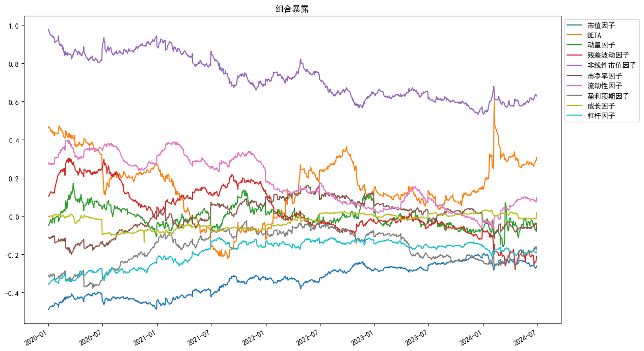

An.plot_returns(factors='style',index_symbol=None,figsize=(15,7))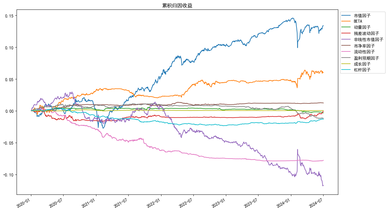

An.plot_exposure_and_returns(factors='style',index_symbol=None,show_factor_perf=False,figsize=(12,6))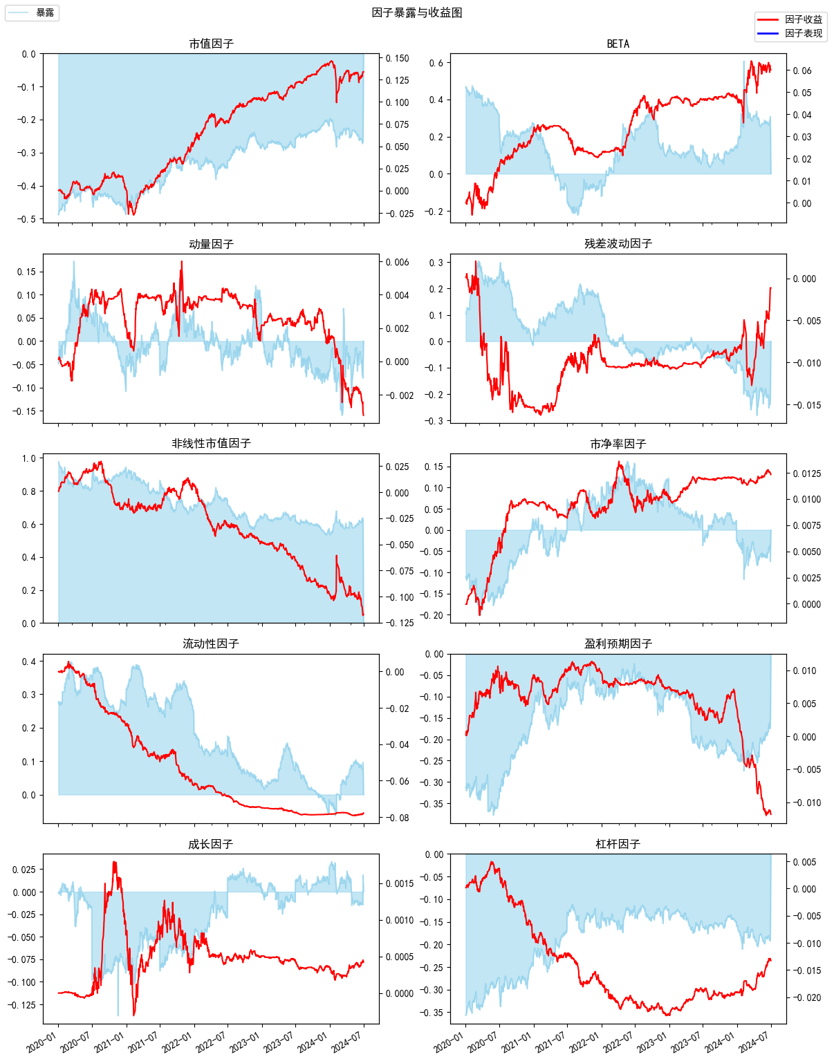

因子数据本地缓存使用示例

具体用法请查看API文档, 此处仅作示例

设置缓存目录

fromjqfactor_analyzer.factor_cacheimportset_cache_dir,get_cache_dir# my_path = 'E:\\jqfactor_cache'# set_cache_dir(my_path) #设置缓存目录为my_pathprint(get_cache_dir()) #输出缓存目录

C:\Users\wq\jqfactor_datacache\bundle

缓存/检查缓存和读取已缓存数据

fromjqfactor_analyzer.factor_cacheimportsave_factor_values_by_group,get_factor_values_by_cache,get_factor_folder,get_cache_dir# import jqdatasdk as jq# jq.auth("账号",'密码') #登陆jqdatasdk来从服务端缓存数据all_factors=jqdatasdk.get_all_factors()
factor_names=all_factors[all_factors.category=='growth'].factor.tolist() #将聚宽因子库中的成长类因子作为一组因子group_name='growth_factors'#因子组名定义为'growth_factors'start_date='2021-01-01'end_date='2021-06-01'# 检查/缓存因子数据factor_path=save_factor_values_by_group(start_date,end_date,factor_names=factor_names,group_name=group_name,overwrite=False,show_progress=True)
# factor_path = os.path.join(get_cache_dir(), get_factor_folder(factor_names,group_name=group_name) #等同于save_factor_values_by_group返回的路径

check/save factor cache : 100%|██████████| 6/6 [00:01<00:00, 5.87it/s]

# 循环获取缓存的因子数据,并拼接trade_days=jqdatasdk.get_trade_days(start_date,end_date)
factor_values= {}
fordateintrade_days:
factor_values[date] =get_factor_values_by_cache(date,codes=None,factor_names=factor_names,group_name=group_name, factor_path=factor_path)#这里实际只需要指定group_name,factor_names参数的其中一个,缓存时指定了group_name时,factor_names不生效factor_values=pd.concat(factor_values)
factor_values.head(5)

.dataframe tbody tr th {
vertical-align: top;
}
.dataframe thead th {
text-align: right;
}

</style>

		financing_cash_growth_rate	net_asset_growth_rate	net_operate_cashflow_growth_rate	net_profit_growth_rate	np_parent_company_owners_growth_rate	operating_revenue_growth_rate	PEG	total_asset_growth_rate	total_profit_growth_rate
	code
2021-01-04	000001.XSHE	4.218607	0.245417	-3.438636	-0.036129	-0.036129	0.139493	NaN	0.172409	-0.053686
	000002.XSHE	-1.059306	0.236022	0.266020	0.009771	0.064828	0.115457	1.229423	0.107217	-0.013790
	000004.XSHE	NaN	11.430834	-0.019530	-3.350306	-3.551808	-0.328126	NaN	10.912087	-3.888289
	000005.XSHE	-1.014341	0.052103	-2.331018	-0.480705	-0.461062	-0.700859	NaN	-0.040798	-0.567470
	000006.XSHE	-0.978757	0.112236	-1.509728	0.083089	0.044869	0.170041	1.931730	-0.005611	0.113066

单因子分析使用示例

具体用法请查看API文档, 此处仅作示例

示例：5日平均换手率因子分析

# 载入函数库importpandasaspdimportjqfactor_analyzerasja# 获取5日平均换手率因子2018-01-01到2018-12-31之间的数据（示例用从库中直接调取）# 聚宽因子库数据获取方法在下方fromjqfactor_analyzer.sampleimportVOL5factor_data=VOL5# 对因子进行分析far=ja.analyze_factor(
factor_data, # factor_data 为因子值的 pandas.DataFramequantiles=10,
periods=(1, 10),
industry='jq_l1',
weight_method='avg',
max_loss=0.1
)
# 获取整理后的因子的IC值far.ic

check/save price cache : 100%|██████████| 13/13 [00:00<00:00, 25.60it/s]
load price info : 100%|██████████| 253/253 [00:06<00:00, 38.09it/s]
load industry info : 100%|██████████| 243/243 [00:00<00:00, 331.46it/s]

.dataframe tbody tr th {
vertical-align: top;
}
.dataframe thead th {
text-align: right;
}

</style>

	period_1	period_10
date
2018-01-02	0.141204	-0.058936
2018-01-03	0.082738	-0.176327
2018-01-04	-0.183788	-0.196901
2018-01-05	0.057023	-0.180102
2018-01-08	-0.025403	-0.187145
...	...	...
2018-12-24	0.098161	-0.198127
2018-12-25	-0.269072	-0.166092
2018-12-26	-0.430034	-0.117108
2018-12-27	-0.107514	-0.040684
2018-12-28	-0.013224	0.039446

243 rows × 2 columns

# 生成统计图表far.create_full_tear_sheet(
demeaned=False, group_adjust=False, by_group=False,
turnover_periods=None, avgretplot=(5, 15), std_bar=False
)

分位数统计

.dataframe tbody tr th {
vertical-align: top;
}
.dataframe thead th {
text-align: right;
}

</style>

	min	max	mean	std	count	count %
factor_quantile
1	0.00000	0.30046	0.072019	0.056611	7293	10.054595
2	0.08846	0.49034	0.198844	0.066169	7266	10.017371
3	0.14954	0.65984	0.309961	0.089310	7219	9.952574
4	0.22594	0.80136	0.423978	0.111141	7248	9.992555
5	0.30904	0.99400	0.553684	0.133578	7280	10.036672
6	0.38860	1.23760	0.696531	0.166341	7211	9.941545
7	0.48394	1.56502	0.874488	0.204828	7240	9.981526
8	0.61900	2.09560	1.132261	0.265739	7226	9.962225
9	0.84984	3.30790	1.639863	0.436992	7261	10.010478
10	1.23172	40.47726	4.276270	3.640945	7290	10.050459

------------------------- 收益分析

.dataframe tbody tr th {
vertical-align: top;
}
.dataframe thead th {
text-align: right;
}

</style>

	period_1	period_10
Ann. alpha	-0.087	-0.060
beta	1.218	1.238
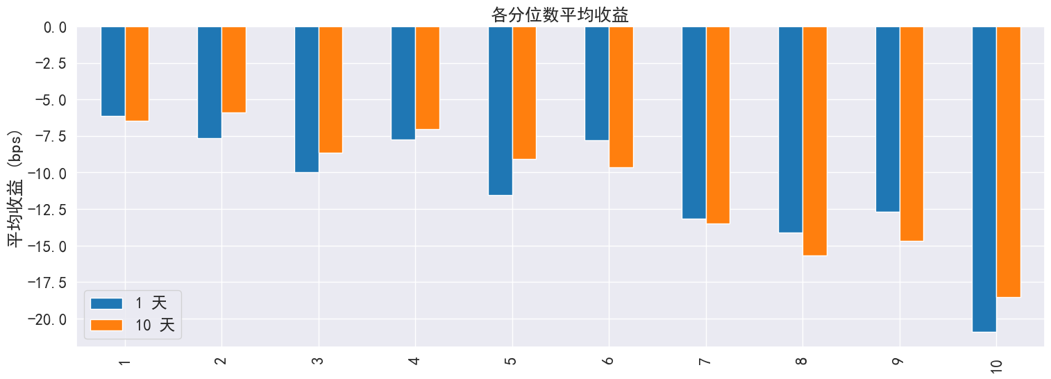
Mean Period Wise Return Top Quantile (bps)	-20.913	-18.530
Mean Period Wise Return Bottom Quantile (bps)	-6.156	-6.452
Mean Period Wise Spread (bps)	-14.757	-13.177

<Figure size 640x480 with 0 Axes>

<Figure size 640x480 with 0 Axes>

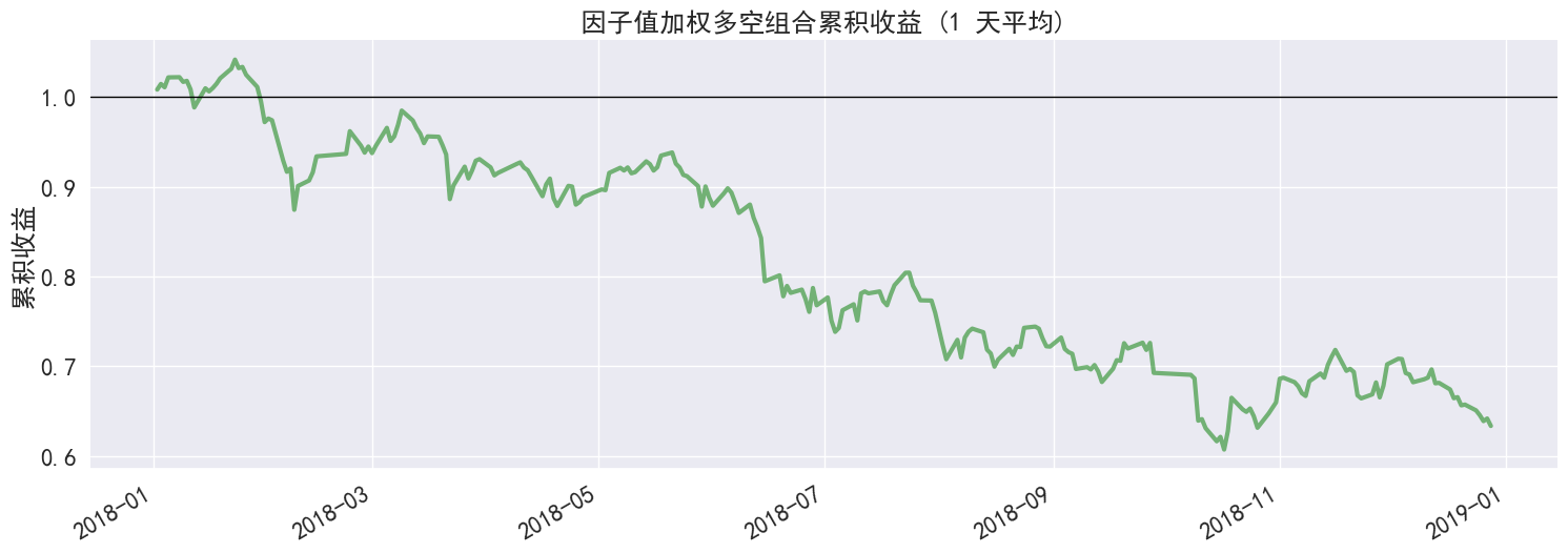
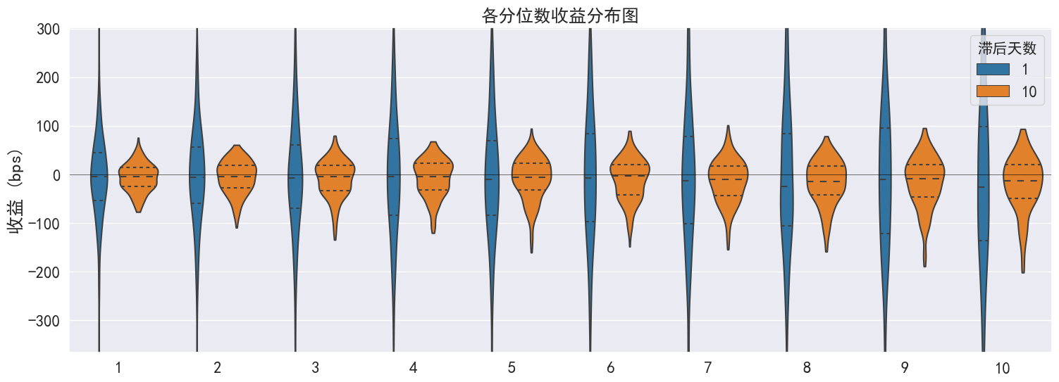
......(图片过多,此处内容演示已省略,请参考api说明使用)

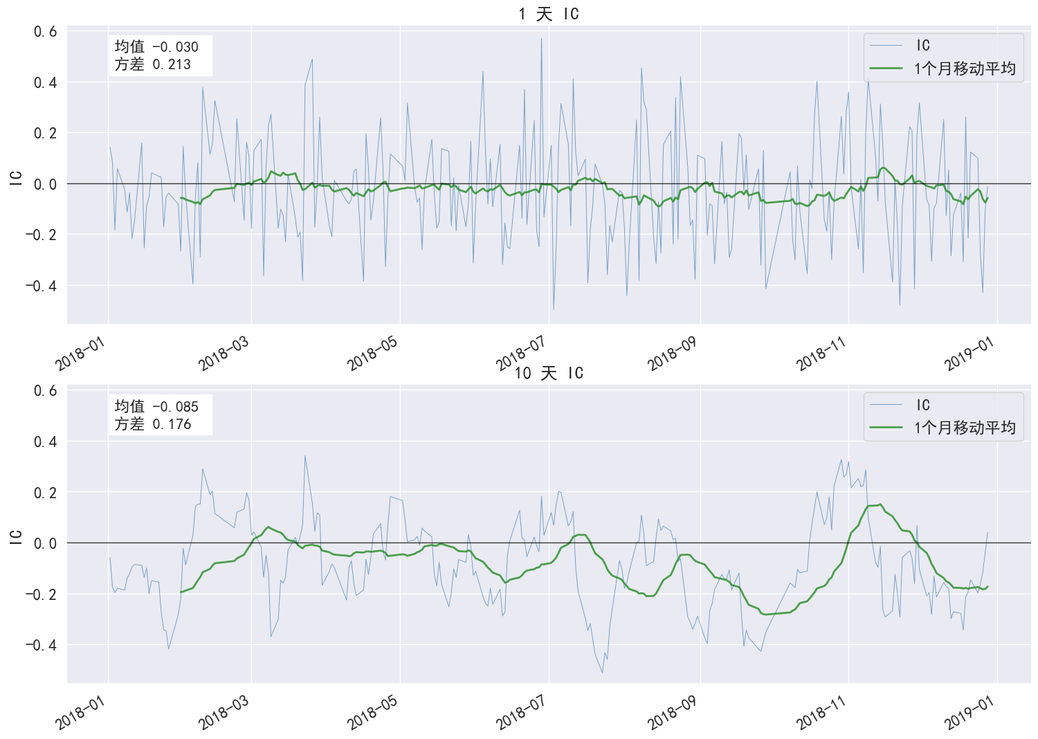
------------------------- IC 分析

.dataframe tbody tr th {
vertical-align: top;
}
.dataframe thead th {
text-align: right;
}

</style>

	period_1	period_10
IC Mean	-0.030	-0.085
IC Std.	0.213	0.176
IR	-0.140	-0.487
t-stat(IC)	-2.180	-7.587
p-value(IC)	0.030	0.000
IC Skew	0.240	0.091
IC Kurtosis	-0.420	-0.485

<Figure size 640x480 with 0 Axes>

<Figure size 640x480 with 0 Axes>

------------------------- 换手率分析

.dataframe tbody tr th {
vertical-align: top;
}
.dataframe thead th {
text-align: right;
}

</style>

	period_1	period_10
Quantile 1 Mean Turnover	0.055	0.222
Quantile 2 Mean Turnover	0.136	0.447
Quantile 3 Mean Turnover	0.206	0.599
Quantile 4 Mean Turnover	0.268	0.680
Quantile 5 Mean Turnover	0.307	0.730
Quantile 6 Mean Turnover	0.337	0.742
Quantile 7 Mean Turnover	0.326	0.735
Quantile 8 Mean Turnover	0.279	0.708
Quantile 9 Mean Turnover	0.196	0.593
Quantile 10 Mean Turnover	0.073	0.283

.dataframe tbody tr th {
vertical-align: top;
}
.dataframe thead th {
text-align: right;
}

</style>

	period_1	period_10
Mean Factor Rank Autocorrelation	0.991	0.884

......(图片过多,此处内容演示已省略,请参考api说明使用)

获取聚宽因子库数据的方法

聚宽因子库包含数百个质量、情绪、风险等其他类目的因子

连接jqdatasdk获取数据包，数据接口需调用聚宽 jqdatasdk 接口获取金融数据 (试用注册地址)

# 获取因子数据：以5日平均换手率为例，该数据可以直接用于因子分析# 具体使用方法可以参照jqdatasdk的API文档importjqdatasdkjqdatasdk.auth('username', 'password')
# 获取聚宽因子库中的VOL5数据factor_data=jqdatasdk.get_factor_values(
securities=jqdatasdk.get_index_stocks('000300.XSHG'),
factors=['VOL5'],
start_date='2018-01-01',
end_date='2018-12-31')['VOL5']

将自有因子值转换成 DataFrame 格式的数据

index 为日期，格式为 pandas 日期通用的 DatetimeIndex
columns 为股票代码，格式要求符合聚宽的代码定义规则（如：平安银行的股票代码为 000001.XSHE）
- 如果是深交所上市的股票，在股票代码后面需要加入 .XSHE
- 如果是上交所上市的股票，在股票代码后面需要加入 .XSHG
将 pandas.DataFrame 转换成满足格式要求数据格式
首先要保证 index 为 DatetimeIndex 格式，一般是通过 pandas 提供的 pandas.to_datetime 函数进行转换，在转换前应确保 index 中的值都为合理的日期格式，如 '2018-01-01' / '20180101'，之后再调用 pandas.to_datetime 进行转换；另外应确保 index 的日期是按照从小到大的顺序排列的，可以通过 sort_index 进行排序；最后请检查 columns 中的股票代码是否都满足聚宽的代码定义。

importpandasaspdsample_data=pd.DataFrame(
[[0.84, 0.43, 2.33, 0.86, 0.96],
[1.06, 0.51, 2.60, 0.90, 1.09],
[1.12, 0.54, 2.68, 0.94, 1.12],
[1.07, 0.64, 2.65, 1.33, 1.15],
[1.21, 0.73, 2.97, 1.65, 1.19]],
index=['2018-01-02', '2018-01-03', '2018-01-04', '2018-01-05', '2018-01-08'],
columns=['000001.XSHE', '000002.XSHE', '000063.XSHE', '000069.XSHE', '000100.XSHE']
)
print(sample_data)
factor_data=sample_data.copy()
# 将 index 转换为 DatetimeIndexfactor_data.index=pd.to_datetime(factor_data.index)
# 将 DataFrame 按照日期顺序排列factor_data=factor_data.sort_index()
# 检查 columns 是否满足聚宽股票代码格式ifnotsample_data.columns.astype(str).str.match('\d{6}\.XSH[EG]').all():
print("有不满足聚宽股票代码格式的股票")
print(sample_data.columns[~sample_data.columns.astype(str).str.match('\d{6}\.XSH[EG]')])
print(factor_data)

将键为日期，值为各股票因子值的 Series 的 dict 转换成 pandas.DataFrame，可以直接利用 pandas.DataFrame 生成

sample_data= \
{'2018-01-02': pd.Seris([0.84, 0.43, 2.33, 0.86, 0.96],
index=['000001.XSHE', '000002.XSHE', '000063.XSHE', '000069.XSHE', '000100.XSHE']),
'2018-01-03': pd.Seris([1.06, 0.51, 2.60, 0.90, 1.09],
index=['000001.XSHE', '000002.XSHE', '000063.XSHE', '000069.XSHE', '000100.XSHE']),
'2018-01-04': pd.Seris([1.12, 0.54, 2.68, 0.94, 1.12],
index=['000001.XSHE', '000002.XSHE', '000063.XSHE', '000069.XSHE', '000100.XSHE']),
'2018-01-05': pd.Seris([1.07, 0.64, 2.65, 1.33, 1.15],
index=['000001.XSHE', '000002.XSHE', '000063.XSHE', '000069.XSHE', '000100.XSHE']),
'2018-01-08': pd.Seris([1.21, 0.73, 2.97, 1.65, 1.19],
index=['000001.XSHE', '000002.XSHE', '000063.XSHE', '000069.XSHE', '000100.XSHE'])}
importpandasaspd# 直接调用 pd.DataFrame 将 dict 转换为 DataFramefactor_data=pd.DataFrame(data).Tprint(factor_data)
# 之后请按照 DataFrae 的方法转换成满足格式要求数据格式

Name		Name	Last commit message	Last commit date
docs		docs
jqfactor_analyzer		jqfactor_analyzer
tests		tests
.gitignore		.gitignore
LICENSE		LICENSE
MANiFEST.in		MANiFEST.in
README.md		README.md
requirements.txt		requirements.txt
setup.cfg		setup.cfg
setup.py		setup.py

Navigation Menu

Uh oh!

Repository files navigation

jqfactor_analyzer

安装

升级

具体使用方法

归因分析使用示例

风格模型的基本概念

使用上述已提供的数据进行归因分析 :

以指数作为基准的归因分析

累积收益的处理

导入模块并登陆 jqdatasdk

处理权重信息

进行归因分析

因子数据本地缓存使用示例

设置缓存目录

缓存/检查缓存和读取已缓存数据

单因子分析使用示例

示例：5日平均换手率因子分析

获取聚宽因子库数据的方法

将自有因子值转换成 DataFrame 格式的数据

About

Releases

Packages

Used by

Contributors

Languages

Uh oh!

Latest commit

History

Folders and files

Repository files navigation

jqfactor_analyzer

安装

升级

具体使用方法

归因分析使用示例

风格模型的基本概念

使用上述已提供的数据进行归因分析 :

以指数作为基准的归因分析

累积收益的处理

导入模块并登陆 jqdatasdk

处理权重信息

进行归因分析

因子数据本地缓存使用示例

设置缓存目录

缓存/检查缓存和读取已缓存数据

单因子分析使用示例

示例：5日平均换手率因子分析

获取聚宽因子库数据的方法

将自有因子值转换成 DataFrame 格式的数据

About

Resources

Stars

Watchers

Forks

Releases

Packages

Used by

Contributors

Languages