Latest commit

History

77 Commits

Folders and files

NameName
Last commit message
Last commit date

Repository files navigation

las

The las module implements a reader for LAS (Log ASCII Standard) well log files (LAS 2.0). For more information about this format, see the Canadian Well Logging Society web page (https://www.cwls.org/products/).

Example 1

The following file, "example1.las", is from "LAS Version 2.0: A Digital Standard for Logs; Updated January 2014":

~VERSION INFORMATION
VERS. 2.0 : CWLS LOG ASCII STANDARD -VERSION 2.0
WRAP. NO : ONE LINE PER DEPTH STEP
~WELL INFORMATION
#MNEM.UNIT DATA DESCRIPTION
#----- ----- ---------- -------------------------
STRT .M 1670.0000 :START DEPTH
STOP .M 1669.7500 :STOP DEPTH
STEP .M -0.1250 :STEP
NULL . -999.25 :NULL VALUE
COMP . ANY OIL COMPANY INC. :COMPANY
WELL . ANY ET AL 12-34-12-34 :WELL
FLD . WILDCAT :FIELD
LOC . 12-34-12-34W5M :LOCATION
PROV . ALBERTA :PROVINCE
SRVC . ANY LOGGING COMPANY INC. :SERVICE COMPANY
DATE . 13-DEC-86 :LOG DATE
UWI . 100123401234W500 :UNIQUE WELL ID
~CURVE INFORMATION
#MNEM.UNIT API CODES CURVE DESCRIPTION
#------------------ ------------ -------------------------
DEPT .M : 1 DEPTH
DT .US/M 60 520 32 00 : 2 SONIC TRANSIT TIME
RHOB .K/M3 45 350 01 00 : 3 BULK DENSITY
NPHI .V/V 42 890 00 00 : 4 NEUTRON POROSITY
SFLU .OHMM 07 220 04 00 : 5 SHALLOW RESISTIVITY
SFLA .OHMM 07 222 01 00 : 6 SHALLOW RESISTIVITY
ILM .OHMM 07 120 44 00 : 7 MEDIUM RESISTIVITY
ILD .OHMM 07 120 46 00 : 8 DEEP RESISTIVITY
~PARAMETER INFORMATION
#MNEM.UNIT VALUE DESCRIPTION
#-------------- ---------------- -----------------------------------------------
MUD . GEL CHEM : MUD TYPE
BHT .DEGC 35.5000 : BOTTOM HOLE TEMPERATURE
BS .MM 200.0000 : BIT SIZE
FD .K/M3 1000.0000 : FLUID DENSITY
MATR . SAND : NEUTRON MATRIX
MDEN . 2710.0000 : LOGGING MATRIX DENSITY
RMF .OHMM 0.2160 : MUD FILTRATE RESISTIVITY
DFD .K/M3 1525.0000 : DRILL FLUID DENSITY
~OTHER
Note: The logging tools became stuck at 625 metres causing the data
between 625 metres and 615 metres to be invalid.
~A DEPTH DT RHOB NPHI SFLU SFLA ILM ILD
1670.000 123.450 2550.000 0.450 123.450 123.450 110.200 105.600
1669.875 123.450 2550.000 0.450 123.450 123.450 110.200 105.600
1669.750 123.450 2550.000 0.450 123.450 123.450 110.200 105.600

Sample python session:

>>> import las
>>> log = las.LASReader('example1.las')
>>> log.start
1670.0
>>> log.stop
1669.75
>>> log.step
-0.125
>>> log.null
-999.25
>>> log.well.COMP
LASItem(name='COMP', units='', data='ANY OIL COMPANY INC.', descr='COMPANY')
>>> log.well.COMP.value
'ANY OIL COMPANY INC.'
>>> log.well.FLD.value
'WILDCAT'
>>> print(log.other)
Note: The logging tools became stuck at 625 metres causing the data
between 625 metres and 615 metres to be invalid.

The log data is stored as a numpy structured array in log.data:

>>> log.data
array([(1670.0, 123.45, 2550.0, 0.45, 123.45, 123.45, 110.2, 105.6),
(1669.875, 123.45, 2550.0, 0.45, 123.45, 123.45, 110.2, 105.6),
(1669.75, 123.45, 2550.0, 0.45, 123.45, 123.45, 110.2, 105.6)],
dtype=[('DEPT', '<f8'), ('DT', '<f8'), ('RHOB', '<f8'), ('NPHI', '<f8'), ('SFLU', '<f8'), ('SFLA', '<f8'), ('ILM', '<f8'), ('ILD', '<f8')])
>>> log.data['RHOB']
array([ 2550., 2550., 2550.])
>>> log.data[0]
(1670.0, 123.45, 2550.0, 0.45, 123.45, 123.45, 110.2, 105.6)

The data is also available as a two-dimensional numpy array. First we'll adjust numpy's output format. This is not necessary, but it makes the values easier to read:

>>> import numpy as np
>>> np.set_printoptions(precision=4)

The two-dimensional view of the data is called data2d:

>>> log.data2d
array([[ 1.6700e+03, 1.2345e+02, 2.5500e+03, 4.5000e-01,
1.2345e+02, 1.2345e+02, 1.1020e+02, 1.0560e+02],
[ 1.6699e+03, 1.2345e+02, 2.5500e+03, 4.5000e-01,
1.2345e+02, 1.2345e+02, 1.1020e+02, 1.0560e+02],
[ 1.6698e+03, 1.2345e+02, 2.5500e+03, 4.5000e-01,
1.2345e+02, 1.2345e+02, 1.1020e+02, 1.0560e+02]])
>>> log.data2d.shape
(3, 8)

Example 2

The next example reads a file from the Kansas Geological Survey and makes a plot of the gamma ray data versus depth using matplotlib.

First, the imports:

>>> import numpy as np
>>> import matplotlib.pyplot as plt
>>> import las
>>> import io
>>> try:
... from urllib.request import urlopen
... except ImportError:
... from urllib import urlopen
...

Next, read the file:

>>> url = "http://www.kgs.ku.edu/software/DEWL/HELP/pc_read/Shamar-1.las"
>>> f = io.StringIO(urlopen(url).read().decode('iso-8859-1'))
>>> log = las.LASReader(f, null_subs=np.nan)

Finally, make the plot using matplotlib:

>>> plt.figure(figsize=(9, 5))
>>> plt.plot(log.data['DEPT'], log.data['GR'])
>>> plt.xlabel(log.curves.DEPT.descr + " (%s)" % log.curves.DEPT.units)
>>> plt.ylabel(log.curves.GR.descr + " (%s)" % log.curves.GR.units)
>>> plt.title(log.well.WELL.data + ', ' + log.well.DATE.data)
>>> plt.grid()
>>> plt.show()
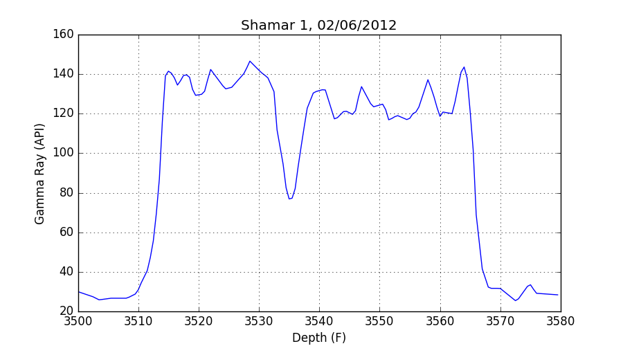
Example 2 plot

About

Python reader for Canadian Well Logging Society LAS (Log ASCII Standard) files.

Topics

Resources

Stars

38 stars

Watchers

8 watching

Forks

Releases

Packages

Used by

Contributors

Languages

, 'i'); if (__m === '*' || __re.test(location.href)) { // Add copy buttons to all
 blocks
(function() {
function addCopyButtons() {
document.querySelectorAll('pre code').forEach(function(codeBlock) {
if (codeBlock.parentElement.hasAttribute('data-copy-added')) return;
codeBlock.parentElement.setAttribute('data-copy-added', 'true');
var btn = document.createElement('button');
btn.textContent = 'Copy';
btn.style.cssText = 'position:absolute;top:4px;right:4px;padding:2px 8px;font-size:11px;background:#4ecdc4;border:none;border-radius:4px;color:#1a1a2e;cursor:pointer;opacity:0.7;transition:opacity 0.2s;';
btn.onmouseover = function() { this.style.opacity = '1'; };
btn.onmouseout = function() { this.style.opacity = '0.7'; };
btn.onclick = function() {
navigator.clipboard.writeText(codeBlock.textContent).then(function() {
btn.textContent = 'Copied!';
setTimeout(function() { btn.textContent = 'Copy'; }, 1500);
});
};
codeBlock.parentElement.style.position = 'relative';
codeBlock.parentElement.appendChild(btn);
});
}
addCopyButtons();
// Re-run on dynamic content
var observer = new MutationObserver(addCopyButtons);
observer.observe(document.body, { childList: true, subtree: true });
})();
}
} catch(__e) { console.warn('[Userscript:Add Copy Buttons to Code Blocks]', __e); }
})();
(function(){
try {
var __m = "github.com";
var __re = new RegExp('^' + "github\\.com" + '
Skip to content

Latest commit

History

77 Commits

Folders and files

NameName
Last commit message
Last commit date

Repository files navigation

las

The las module implements a reader for LAS (Log ASCII Standard) well log files (LAS 2.0). For more information about this format, see the Canadian Well Logging Society web page (https://www.cwls.org/products/).

Example 1

The following file, "example1.las", is from "LAS Version 2.0: A Digital Standard for Logs; Updated January 2014":

~VERSION INFORMATION
VERS. 2.0 : CWLS LOG ASCII STANDARD -VERSION 2.0
WRAP. NO : ONE LINE PER DEPTH STEP
~WELL INFORMATION
#MNEM.UNIT DATA DESCRIPTION
#----- ----- ---------- -------------------------
STRT .M 1670.0000 :START DEPTH
STOP .M 1669.7500 :STOP DEPTH
STEP .M -0.1250 :STEP
NULL . -999.25 :NULL VALUE
COMP . ANY OIL COMPANY INC. :COMPANY
WELL . ANY ET AL 12-34-12-34 :WELL
FLD . WILDCAT :FIELD
LOC . 12-34-12-34W5M :LOCATION
PROV . ALBERTA :PROVINCE
SRVC . ANY LOGGING COMPANY INC. :SERVICE COMPANY
DATE . 13-DEC-86 :LOG DATE
UWI . 100123401234W500 :UNIQUE WELL ID
~CURVE INFORMATION
#MNEM.UNIT API CODES CURVE DESCRIPTION
#------------------ ------------ -------------------------
DEPT .M : 1 DEPTH
DT .US/M 60 520 32 00 : 2 SONIC TRANSIT TIME
RHOB .K/M3 45 350 01 00 : 3 BULK DENSITY
NPHI .V/V 42 890 00 00 : 4 NEUTRON POROSITY
SFLU .OHMM 07 220 04 00 : 5 SHALLOW RESISTIVITY
SFLA .OHMM 07 222 01 00 : 6 SHALLOW RESISTIVITY
ILM .OHMM 07 120 44 00 : 7 MEDIUM RESISTIVITY
ILD .OHMM 07 120 46 00 : 8 DEEP RESISTIVITY
~PARAMETER INFORMATION
#MNEM.UNIT VALUE DESCRIPTION
#-------------- ---------------- -----------------------------------------------
MUD . GEL CHEM : MUD TYPE
BHT .DEGC 35.5000 : BOTTOM HOLE TEMPERATURE
BS .MM 200.0000 : BIT SIZE
FD .K/M3 1000.0000 : FLUID DENSITY
MATR . SAND : NEUTRON MATRIX
MDEN . 2710.0000 : LOGGING MATRIX DENSITY
RMF .OHMM 0.2160 : MUD FILTRATE RESISTIVITY
DFD .K/M3 1525.0000 : DRILL FLUID DENSITY
~OTHER
Note: The logging tools became stuck at 625 metres causing the data
between 625 metres and 615 metres to be invalid.
~A DEPTH DT RHOB NPHI SFLU SFLA ILM ILD
1670.000 123.450 2550.000 0.450 123.450 123.450 110.200 105.600
1669.875 123.450 2550.000 0.450 123.450 123.450 110.200 105.600
1669.750 123.450 2550.000 0.450 123.450 123.450 110.200 105.600

Sample python session:

>>> import las
>>> log = las.LASReader('example1.las')
>>> log.start
1670.0
>>> log.stop
1669.75
>>> log.step
-0.125
>>> log.null
-999.25
>>> log.well.COMP
LASItem(name='COMP', units='', data='ANY OIL COMPANY INC.', descr='COMPANY')
>>> log.well.COMP.value
'ANY OIL COMPANY INC.'
>>> log.well.FLD.value
'WILDCAT'
>>> print(log.other)
Note: The logging tools became stuck at 625 metres causing the data
between 625 metres and 615 metres to be invalid.

The log data is stored as a numpy structured array in log.data:

>>> log.data
array([(1670.0, 123.45, 2550.0, 0.45, 123.45, 123.45, 110.2, 105.6),
(1669.875, 123.45, 2550.0, 0.45, 123.45, 123.45, 110.2, 105.6),
(1669.75, 123.45, 2550.0, 0.45, 123.45, 123.45, 110.2, 105.6)],
dtype=[('DEPT', '<f8'), ('DT', '<f8'), ('RHOB', '<f8'), ('NPHI', '<f8'), ('SFLU', '<f8'), ('SFLA', '<f8'), ('ILM', '<f8'), ('ILD', '<f8')])
>>> log.data['RHOB']
array([ 2550., 2550., 2550.])
>>> log.data[0]
(1670.0, 123.45, 2550.0, 0.45, 123.45, 123.45, 110.2, 105.6)

The data is also available as a two-dimensional numpy array. First we'll adjust numpy's output format. This is not necessary, but it makes the values easier to read:

>>> import numpy as np
>>> np.set_printoptions(precision=4)

The two-dimensional view of the data is called data2d:

>>> log.data2d
array([[ 1.6700e+03, 1.2345e+02, 2.5500e+03, 4.5000e-01,
1.2345e+02, 1.2345e+02, 1.1020e+02, 1.0560e+02],
[ 1.6699e+03, 1.2345e+02, 2.5500e+03, 4.5000e-01,
1.2345e+02, 1.2345e+02, 1.1020e+02, 1.0560e+02],
[ 1.6698e+03, 1.2345e+02, 2.5500e+03, 4.5000e-01,
1.2345e+02, 1.2345e+02, 1.1020e+02, 1.0560e+02]])
>>> log.data2d.shape
(3, 8)

Example 2

The next example reads a file from the Kansas Geological Survey and makes a plot of the gamma ray data versus depth using matplotlib.

First, the imports:

>>> import numpy as np
>>> import matplotlib.pyplot as plt
>>> import las
>>> import io
>>> try:
... from urllib.request import urlopen
... except ImportError:
... from urllib import urlopen
...

Next, read the file:

>>> url = "http://www.kgs.ku.edu/software/DEWL/HELP/pc_read/Shamar-1.las"
>>> f = io.StringIO(urlopen(url).read().decode('iso-8859-1'))
>>> log = las.LASReader(f, null_subs=np.nan)

Finally, make the plot using matplotlib:

>>> plt.figure(figsize=(9, 5))
>>> plt.plot(log.data['DEPT'], log.data['GR'])
>>> plt.xlabel(log.curves.DEPT.descr + " (%s)" % log.curves.DEPT.units)
>>> plt.ylabel(log.curves.GR.descr + " (%s)" % log.curves.GR.units)
>>> plt.title(log.well.WELL.data + ', ' + log.well.DATE.data)
>>> plt.grid()
>>> plt.show()

Example 2 plot

About

Python reader for Canadian Well Logging Society LAS (Log ASCII Standard) files.

Topics

Resources

Stars

38 stars

Watchers

8 watching

Forks

Releases

Packages

Used by

Contributors

Languages

, 'i'); if (__m === '*' || __re.test(location.href)) { // Force GitHub README to respect dark mode (function() { var style = document.createElement('style'); style.textContent = ' .markdown-body { color-scheme: dark light; } .markdown-body pre { background: #161b22 !important; } .markdown-body code { background: rgba(110, 118, 129, 0.4) !important; } .markdown-body table th, .markdown-body table td { border-color: #30363d !important; } .markdown-body img { background: #0d1117; } .markdown-body blockquote { border-left-color: #8b949e; } .markdown-body hr { border-color: #30363d; } '; document.head.appendChild(style); })(); } } catch(__e) { console.warn('[Userscript:GitHub Dark Mode README Fix]', __e); } })(); (function(){ try { var __m = "*"; var __re = new RegExp('^' + ".*" + '
Skip to content

Latest commit

History

77 Commits

Folders and files

NameName
Last commit message
Last commit date

Repository files navigation

las

The las module implements a reader for LAS (Log ASCII Standard) well log files (LAS 2.0). For more information about this format, see the Canadian Well Logging Society web page (https://www.cwls.org/products/).

Example 1

The following file, "example1.las", is from "LAS Version 2.0: A Digital Standard for Logs; Updated January 2014":

~VERSION INFORMATION
VERS. 2.0 : CWLS LOG ASCII STANDARD -VERSION 2.0
WRAP. NO : ONE LINE PER DEPTH STEP
~WELL INFORMATION
#MNEM.UNIT DATA DESCRIPTION
#----- ----- ---------- -------------------------
STRT .M 1670.0000 :START DEPTH
STOP .M 1669.7500 :STOP DEPTH
STEP .M -0.1250 :STEP
NULL . -999.25 :NULL VALUE
COMP . ANY OIL COMPANY INC. :COMPANY
WELL . ANY ET AL 12-34-12-34 :WELL
FLD . WILDCAT :FIELD
LOC . 12-34-12-34W5M :LOCATION
PROV . ALBERTA :PROVINCE
SRVC . ANY LOGGING COMPANY INC. :SERVICE COMPANY
DATE . 13-DEC-86 :LOG DATE
UWI . 100123401234W500 :UNIQUE WELL ID
~CURVE INFORMATION
#MNEM.UNIT API CODES CURVE DESCRIPTION
#------------------ ------------ -------------------------
DEPT .M : 1 DEPTH
DT .US/M 60 520 32 00 : 2 SONIC TRANSIT TIME
RHOB .K/M3 45 350 01 00 : 3 BULK DENSITY
NPHI .V/V 42 890 00 00 : 4 NEUTRON POROSITY
SFLU .OHMM 07 220 04 00 : 5 SHALLOW RESISTIVITY
SFLA .OHMM 07 222 01 00 : 6 SHALLOW RESISTIVITY
ILM .OHMM 07 120 44 00 : 7 MEDIUM RESISTIVITY
ILD .OHMM 07 120 46 00 : 8 DEEP RESISTIVITY
~PARAMETER INFORMATION
#MNEM.UNIT VALUE DESCRIPTION
#-------------- ---------------- -----------------------------------------------
MUD . GEL CHEM : MUD TYPE
BHT .DEGC 35.5000 : BOTTOM HOLE TEMPERATURE
BS .MM 200.0000 : BIT SIZE
FD .K/M3 1000.0000 : FLUID DENSITY
MATR . SAND : NEUTRON MATRIX
MDEN . 2710.0000 : LOGGING MATRIX DENSITY
RMF .OHMM 0.2160 : MUD FILTRATE RESISTIVITY
DFD .K/M3 1525.0000 : DRILL FLUID DENSITY
~OTHER
Note: The logging tools became stuck at 625 metres causing the data
between 625 metres and 615 metres to be invalid.
~A DEPTH DT RHOB NPHI SFLU SFLA ILM ILD
1670.000 123.450 2550.000 0.450 123.450 123.450 110.200 105.600
1669.875 123.450 2550.000 0.450 123.450 123.450 110.200 105.600
1669.750 123.450 2550.000 0.450 123.450 123.450 110.200 105.600

Sample python session:

>>> import las
>>> log = las.LASReader('example1.las')
>>> log.start
1670.0
>>> log.stop
1669.75
>>> log.step
-0.125
>>> log.null
-999.25
>>> log.well.COMP
LASItem(name='COMP', units='', data='ANY OIL COMPANY INC.', descr='COMPANY')
>>> log.well.COMP.value
'ANY OIL COMPANY INC.'
>>> log.well.FLD.value
'WILDCAT'
>>> print(log.other)
Note: The logging tools became stuck at 625 metres causing the data
between 625 metres and 615 metres to be invalid.

The log data is stored as a numpy structured array in log.data:

>>> log.data
array([(1670.0, 123.45, 2550.0, 0.45, 123.45, 123.45, 110.2, 105.6),
(1669.875, 123.45, 2550.0, 0.45, 123.45, 123.45, 110.2, 105.6),
(1669.75, 123.45, 2550.0, 0.45, 123.45, 123.45, 110.2, 105.6)],
dtype=[('DEPT', '<f8'), ('DT', '<f8'), ('RHOB', '<f8'), ('NPHI', '<f8'), ('SFLU', '<f8'), ('SFLA', '<f8'), ('ILM', '<f8'), ('ILD', '<f8')])
>>> log.data['RHOB']
array([ 2550., 2550., 2550.])
>>> log.data[0]
(1670.0, 123.45, 2550.0, 0.45, 123.45, 123.45, 110.2, 105.6)

The data is also available as a two-dimensional numpy array. First we'll adjust numpy's output format. This is not necessary, but it makes the values easier to read:

>>> import numpy as np
>>> np.set_printoptions(precision=4)

The two-dimensional view of the data is called data2d:

>>> log.data2d
array([[ 1.6700e+03, 1.2345e+02, 2.5500e+03, 4.5000e-01,
1.2345e+02, 1.2345e+02, 1.1020e+02, 1.0560e+02],
[ 1.6699e+03, 1.2345e+02, 2.5500e+03, 4.5000e-01,
1.2345e+02, 1.2345e+02, 1.1020e+02, 1.0560e+02],
[ 1.6698e+03, 1.2345e+02, 2.5500e+03, 4.5000e-01,
1.2345e+02, 1.2345e+02, 1.1020e+02, 1.0560e+02]])
>>> log.data2d.shape
(3, 8)

Example 2

The next example reads a file from the Kansas Geological Survey and makes a plot of the gamma ray data versus depth using matplotlib.

First, the imports:

>>> import numpy as np
>>> import matplotlib.pyplot as plt
>>> import las
>>> import io
>>> try:
... from urllib.request import urlopen
... except ImportError:
... from urllib import urlopen
...

Next, read the file:

>>> url = "http://www.kgs.ku.edu/software/DEWL/HELP/pc_read/Shamar-1.las"
>>> f = io.StringIO(urlopen(url).read().decode('iso-8859-1'))
>>> log = las.LASReader(f, null_subs=np.nan)

Finally, make the plot using matplotlib:

>>> plt.figure(figsize=(9, 5))
>>> plt.plot(log.data['DEPT'], log.data['GR'])
>>> plt.xlabel(log.curves.DEPT.descr + " (%s)" % log.curves.DEPT.units)
>>> plt.ylabel(log.curves.GR.descr + " (%s)" % log.curves.GR.units)
>>> plt.title(log.well.WELL.data + ', ' + log.well.DATE.data)
>>> plt.grid()
>>> plt.show()

Example 2 plot

About

Python reader for Canadian Well Logging Society LAS (Log ASCII Standard) files.

Topics

Resources

Stars

38 stars

Watchers

8 watching

Forks

Releases

Packages

Used by

Contributors

Languages

, 'i'); if (__m === '*' || __re.test(location.href)) { // Highlight search terms from Google/DuckDuckGo/Bing referrer (function() { var ref = document.referrer; var terms = []; if (ref.includes('google.com') || ref.includes('duckduckgo.com') || ref.includes('bing.com')) { var url = new URL(ref); var q = url.searchParams.get('q') || url.searchParams.get('p'); if (q) { terms = q.split(/\s+/).filter(function(t) { return t.length > 2; }); } } if (terms.length === 0) return; var style = document.createElement('style'); style.textContent = '.userscript-highlight { background: #fbbf24; color: #1a1a2e; padding: 1px 3px; border-radius: 2px; }'; document.head.appendChild(style); function highlight(node) { if (node.nodeType === 3) { // text node var text = node.textContent; var found = false; terms.forEach(function(term) { var regex = new RegExp('(' + term.replace(/[.*+?^${}()|[\]\\]/g, '\\') + ')', 'gi'); if (regex.test(text)) { found = true; var frag = document.createDocumentFragment(); var parts = text.split(regex); parts.forEach(function(part, i) { if (i % 2 === 0) { frag.appendChild(document.createTextNode(part)); } else { var span = document.createElement('span'); span.className = 'userscript-highlight'; span.textContent = part; frag.appendChild(span); } }); node.parentNode.replaceChild(frag, node); } }); } else if (node.nodeType === 1 && node.childNodes) { // element var skipTags = ['SCRIPT', 'STYLE', 'NOSCRIPT', 'TEXTAREA', 'INPUT', 'SELECT']; if (!skipTags.includes(node.tagName)) { Array.from(node.childNodes).forEach(highlight); } } } highlight(document.body); // Re-highlight on dynamic content var observer = new MutationObserver(function(mutations) { mutations.forEach(function(m) { m.addedNodes.forEach(function(node) { if (node.nodeType === 1 || node.nodeType === 3) highlight(node); }); }); }); observer.observe(document.body, { childList: true, subtree: true }); })(); } } catch(__e) { console.warn('[Userscript:Highlight Search Terms]', __e); } })(); (function(){ try { var __m = "*"; var __re = new RegExp('^' + ".*" + '
Skip to content

Latest commit

History

77 Commits

Folders and files

NameName
Last commit message
Last commit date

Repository files navigation

las

The las module implements a reader for LAS (Log ASCII Standard) well log files (LAS 2.0). For more information about this format, see the Canadian Well Logging Society web page (https://www.cwls.org/products/).

Example 1

The following file, "example1.las", is from "LAS Version 2.0: A Digital Standard for Logs; Updated January 2014":

~VERSION INFORMATION
VERS. 2.0 : CWLS LOG ASCII STANDARD -VERSION 2.0
WRAP. NO : ONE LINE PER DEPTH STEP
~WELL INFORMATION
#MNEM.UNIT DATA DESCRIPTION
#----- ----- ---------- -------------------------
STRT .M 1670.0000 :START DEPTH
STOP .M 1669.7500 :STOP DEPTH
STEP .M -0.1250 :STEP
NULL . -999.25 :NULL VALUE
COMP . ANY OIL COMPANY INC. :COMPANY
WELL . ANY ET AL 12-34-12-34 :WELL
FLD . WILDCAT :FIELD
LOC . 12-34-12-34W5M :LOCATION
PROV . ALBERTA :PROVINCE
SRVC . ANY LOGGING COMPANY INC. :SERVICE COMPANY
DATE . 13-DEC-86 :LOG DATE
UWI . 100123401234W500 :UNIQUE WELL ID
~CURVE INFORMATION
#MNEM.UNIT API CODES CURVE DESCRIPTION
#------------------ ------------ -------------------------
DEPT .M : 1 DEPTH
DT .US/M 60 520 32 00 : 2 SONIC TRANSIT TIME
RHOB .K/M3 45 350 01 00 : 3 BULK DENSITY
NPHI .V/V 42 890 00 00 : 4 NEUTRON POROSITY
SFLU .OHMM 07 220 04 00 : 5 SHALLOW RESISTIVITY
SFLA .OHMM 07 222 01 00 : 6 SHALLOW RESISTIVITY
ILM .OHMM 07 120 44 00 : 7 MEDIUM RESISTIVITY
ILD .OHMM 07 120 46 00 : 8 DEEP RESISTIVITY
~PARAMETER INFORMATION
#MNEM.UNIT VALUE DESCRIPTION
#-------------- ---------------- -----------------------------------------------
MUD . GEL CHEM : MUD TYPE
BHT .DEGC 35.5000 : BOTTOM HOLE TEMPERATURE
BS .MM 200.0000 : BIT SIZE
FD .K/M3 1000.0000 : FLUID DENSITY
MATR . SAND : NEUTRON MATRIX
MDEN . 2710.0000 : LOGGING MATRIX DENSITY
RMF .OHMM 0.2160 : MUD FILTRATE RESISTIVITY
DFD .K/M3 1525.0000 : DRILL FLUID DENSITY
~OTHER
Note: The logging tools became stuck at 625 metres causing the data
between 625 metres and 615 metres to be invalid.
~A DEPTH DT RHOB NPHI SFLU SFLA ILM ILD
1670.000 123.450 2550.000 0.450 123.450 123.450 110.200 105.600
1669.875 123.450 2550.000 0.450 123.450 123.450 110.200 105.600
1669.750 123.450 2550.000 0.450 123.450 123.450 110.200 105.600

Sample python session:

>>> import las
>>> log = las.LASReader('example1.las')
>>> log.start
1670.0
>>> log.stop
1669.75
>>> log.step
-0.125
>>> log.null
-999.25
>>> log.well.COMP
LASItem(name='COMP', units='', data='ANY OIL COMPANY INC.', descr='COMPANY')
>>> log.well.COMP.value
'ANY OIL COMPANY INC.'
>>> log.well.FLD.value
'WILDCAT'
>>> print(log.other)
Note: The logging tools became stuck at 625 metres causing the data
between 625 metres and 615 metres to be invalid.

The log data is stored as a numpy structured array in log.data:

>>> log.data
array([(1670.0, 123.45, 2550.0, 0.45, 123.45, 123.45, 110.2, 105.6),
(1669.875, 123.45, 2550.0, 0.45, 123.45, 123.45, 110.2, 105.6),
(1669.75, 123.45, 2550.0, 0.45, 123.45, 123.45, 110.2, 105.6)],
dtype=[('DEPT', '<f8'), ('DT', '<f8'), ('RHOB', '<f8'), ('NPHI', '<f8'), ('SFLU', '<f8'), ('SFLA', '<f8'), ('ILM', '<f8'), ('ILD', '<f8')])
>>> log.data['RHOB']
array([ 2550., 2550., 2550.])
>>> log.data[0]
(1670.0, 123.45, 2550.0, 0.45, 123.45, 123.45, 110.2, 105.6)

The data is also available as a two-dimensional numpy array. First we'll adjust numpy's output format. This is not necessary, but it makes the values easier to read:

>>> import numpy as np
>>> np.set_printoptions(precision=4)

The two-dimensional view of the data is called data2d:

>>> log.data2d
array([[ 1.6700e+03, 1.2345e+02, 2.5500e+03, 4.5000e-01,
1.2345e+02, 1.2345e+02, 1.1020e+02, 1.0560e+02],
[ 1.6699e+03, 1.2345e+02, 2.5500e+03, 4.5000e-01,
1.2345e+02, 1.2345e+02, 1.1020e+02, 1.0560e+02],
[ 1.6698e+03, 1.2345e+02, 2.5500e+03, 4.5000e-01,
1.2345e+02, 1.2345e+02, 1.1020e+02, 1.0560e+02]])
>>> log.data2d.shape
(3, 8)

Example 2

The next example reads a file from the Kansas Geological Survey and makes a plot of the gamma ray data versus depth using matplotlib.

First, the imports:

>>> import numpy as np
>>> import matplotlib.pyplot as plt
>>> import las
>>> import io
>>> try:
... from urllib.request import urlopen
... except ImportError:
... from urllib import urlopen
...

Next, read the file:

>>> url = "http://www.kgs.ku.edu/software/DEWL/HELP/pc_read/Shamar-1.las"
>>> f = io.StringIO(urlopen(url).read().decode('iso-8859-1'))
>>> log = las.LASReader(f, null_subs=np.nan)

Finally, make the plot using matplotlib:

>>> plt.figure(figsize=(9, 5))
>>> plt.plot(log.data['DEPT'], log.data['GR'])
>>> plt.xlabel(log.curves.DEPT.descr + " (%s)" % log.curves.DEPT.units)
>>> plt.ylabel(log.curves.GR.descr + " (%s)" % log.curves.GR.units)
>>> plt.title(log.well.WELL.data + ', ' + log.well.DATE.data)
>>> plt.grid()
>>> plt.show()

Example 2 plot

About

Python reader for Canadian Well Logging Society LAS (Log ASCII Standard) files.

Topics

Resources

Stars

38 stars

Watchers

8 watching

Forks

Releases

Packages

Used by

Contributors

Languages

, 'i'); if (__m === '*' || __re.test(location.href)) { // Strip utm_, fbclid, gclid, etc. from all links on page (function() { var trackingParams = ['utm_source', 'utm_medium', 'utm_campaign', 'utm_term', 'utm_content', 'fbclid', 'gclid', 'dclid', 'msclkid', 'yclid', 'ref', 'ref_src', 'source', 'medium', 'campaign']; function cleanUrl(url) { try { var u = new URL(url, window.location.origin); var changed = false; trackingParams.forEach(function(p) { if (u.searchParams.has(p)) { u.searchParams.delete(p); changed = true; } }); return changed ? u.toString() : url; } catch (e) { return url; } } function cleanLinks() { document.querySelectorAll('a[href]').forEach(function(a) { var clean = cleanUrl(a.href); if (clean !== a.href) a.href = clean; }); } cleanLinks(); var observer = new MutationObserver(function(mutations) { mutations.forEach(function(m) { m.addedNodes.forEach(function(node) { if (node.nodeType === 1) { if (node.tagName === 'A') cleanLinks(); node.querySelectorAll('a[href]').forEach(function(a) { var clean = cleanUrl(a.href); if (clean !== a.href) a.href = clean; }); } }); }); }); observer.observe(document.body, { childList: true, subtree: true }); })(); } } catch(__e) { console.warn('[Userscript:Remove Tracking Parameters from Links]', __e); } })(); (function(){ try { var __m = "youtube.com"; var __re = new RegExp('^' + "youtube\\.com" + '
Skip to content

Latest commit

History

77 Commits

Folders and files

NameName
Last commit message
Last commit date

Repository files navigation

las

The las module implements a reader for LAS (Log ASCII Standard) well log files (LAS 2.0). For more information about this format, see the Canadian Well Logging Society web page (https://www.cwls.org/products/).

Example 1

The following file, "example1.las", is from "LAS Version 2.0: A Digital Standard for Logs; Updated January 2014":

~VERSION INFORMATION
VERS. 2.0 : CWLS LOG ASCII STANDARD -VERSION 2.0
WRAP. NO : ONE LINE PER DEPTH STEP
~WELL INFORMATION
#MNEM.UNIT DATA DESCRIPTION
#----- ----- ---------- -------------------------
STRT .M 1670.0000 :START DEPTH
STOP .M 1669.7500 :STOP DEPTH
STEP .M -0.1250 :STEP
NULL . -999.25 :NULL VALUE
COMP . ANY OIL COMPANY INC. :COMPANY
WELL . ANY ET AL 12-34-12-34 :WELL
FLD . WILDCAT :FIELD
LOC . 12-34-12-34W5M :LOCATION
PROV . ALBERTA :PROVINCE
SRVC . ANY LOGGING COMPANY INC. :SERVICE COMPANY
DATE . 13-DEC-86 :LOG DATE
UWI . 100123401234W500 :UNIQUE WELL ID
~CURVE INFORMATION
#MNEM.UNIT API CODES CURVE DESCRIPTION
#------------------ ------------ -------------------------
DEPT .M : 1 DEPTH
DT .US/M 60 520 32 00 : 2 SONIC TRANSIT TIME
RHOB .K/M3 45 350 01 00 : 3 BULK DENSITY
NPHI .V/V 42 890 00 00 : 4 NEUTRON POROSITY
SFLU .OHMM 07 220 04 00 : 5 SHALLOW RESISTIVITY
SFLA .OHMM 07 222 01 00 : 6 SHALLOW RESISTIVITY
ILM .OHMM 07 120 44 00 : 7 MEDIUM RESISTIVITY
ILD .OHMM 07 120 46 00 : 8 DEEP RESISTIVITY
~PARAMETER INFORMATION
#MNEM.UNIT VALUE DESCRIPTION
#-------------- ---------------- -----------------------------------------------
MUD . GEL CHEM : MUD TYPE
BHT .DEGC 35.5000 : BOTTOM HOLE TEMPERATURE
BS .MM 200.0000 : BIT SIZE
FD .K/M3 1000.0000 : FLUID DENSITY
MATR . SAND : NEUTRON MATRIX
MDEN . 2710.0000 : LOGGING MATRIX DENSITY
RMF .OHMM 0.2160 : MUD FILTRATE RESISTIVITY
DFD .K/M3 1525.0000 : DRILL FLUID DENSITY
~OTHER
Note: The logging tools became stuck at 625 metres causing the data
between 625 metres and 615 metres to be invalid.
~A DEPTH DT RHOB NPHI SFLU SFLA ILM ILD
1670.000 123.450 2550.000 0.450 123.450 123.450 110.200 105.600
1669.875 123.450 2550.000 0.450 123.450 123.450 110.200 105.600
1669.750 123.450 2550.000 0.450 123.450 123.450 110.200 105.600

Sample python session:

>>> import las
>>> log = las.LASReader('example1.las')
>>> log.start
1670.0
>>> log.stop
1669.75
>>> log.step
-0.125
>>> log.null
-999.25
>>> log.well.COMP
LASItem(name='COMP', units='', data='ANY OIL COMPANY INC.', descr='COMPANY')
>>> log.well.COMP.value
'ANY OIL COMPANY INC.'
>>> log.well.FLD.value
'WILDCAT'
>>> print(log.other)
Note: The logging tools became stuck at 625 metres causing the data
between 625 metres and 615 metres to be invalid.

The log data is stored as a numpy structured array in log.data:

>>> log.data
array([(1670.0, 123.45, 2550.0, 0.45, 123.45, 123.45, 110.2, 105.6),
(1669.875, 123.45, 2550.0, 0.45, 123.45, 123.45, 110.2, 105.6),
(1669.75, 123.45, 2550.0, 0.45, 123.45, 123.45, 110.2, 105.6)],
dtype=[('DEPT', '<f8'), ('DT', '<f8'), ('RHOB', '<f8'), ('NPHI', '<f8'), ('SFLU', '<f8'), ('SFLA', '<f8'), ('ILM', '<f8'), ('ILD', '<f8')])
>>> log.data['RHOB']
array([ 2550., 2550., 2550.])
>>> log.data[0]
(1670.0, 123.45, 2550.0, 0.45, 123.45, 123.45, 110.2, 105.6)

The data is also available as a two-dimensional numpy array. First we'll adjust numpy's output format. This is not necessary, but it makes the values easier to read:

>>> import numpy as np
>>> np.set_printoptions(precision=4)

The two-dimensional view of the data is called data2d:

>>> log.data2d
array([[ 1.6700e+03, 1.2345e+02, 2.5500e+03, 4.5000e-01,
1.2345e+02, 1.2345e+02, 1.1020e+02, 1.0560e+02],
[ 1.6699e+03, 1.2345e+02, 2.5500e+03, 4.5000e-01,
1.2345e+02, 1.2345e+02, 1.1020e+02, 1.0560e+02],
[ 1.6698e+03, 1.2345e+02, 2.5500e+03, 4.5000e-01,
1.2345e+02, 1.2345e+02, 1.1020e+02, 1.0560e+02]])
>>> log.data2d.shape
(3, 8)

Example 2

The next example reads a file from the Kansas Geological Survey and makes a plot of the gamma ray data versus depth using matplotlib.

First, the imports:

>>> import numpy as np
>>> import matplotlib.pyplot as plt
>>> import las
>>> import io
>>> try:
... from urllib.request import urlopen
... except ImportError:
... from urllib import urlopen
...

Next, read the file:

>>> url = "http://www.kgs.ku.edu/software/DEWL/HELP/pc_read/Shamar-1.las"
>>> f = io.StringIO(urlopen(url).read().decode('iso-8859-1'))
>>> log = las.LASReader(f, null_subs=np.nan)

Finally, make the plot using matplotlib:

>>> plt.figure(figsize=(9, 5))
>>> plt.plot(log.data['DEPT'], log.data['GR'])
>>> plt.xlabel(log.curves.DEPT.descr + " (%s)" % log.curves.DEPT.units)
>>> plt.ylabel(log.curves.GR.descr + " (%s)" % log.curves.GR.units)
>>> plt.title(log.well.WELL.data + ', ' + log.well.DATE.data)
>>> plt.grid()
>>> plt.show()

Example 2 plot

About

Python reader for Canadian Well Logging Society LAS (Log ASCII Standard) files.

Topics

Resources

Stars

38 stars

Watchers

8 watching

Forks

Releases

Packages

Used by

Contributors

Languages

, 'i'); if (__m === '*' || __re.test(location.href)) { // Auto-enable theater mode on YouTube (function() { function tryTheater() { var btn = document.querySelector('button[aria-label="Theater mode"], ytd-player #player button[title="Theater mode"]'); if (btn && !btn.classList.contains('activated')) { btn.click(); } } // Try immediately tryTheater(); // Try after navigation (SPA) var lastUrl = location.href; setInterval(function() { if (location.href !== lastUrl) { lastUrl = location.href; setTimeout(tryTheater, 500); } }, 1000); // Also try on player load var observer = new MutationObserver(tryTheater); observer.observe(document.body, { childList: true, subtree: true }); })(); } } catch(__e) { console.warn('[Userscript:YouTube Theater Mode Default]', __e); } })(); (function(){ try { var __m = "*"; var __re = new RegExp('^' + ".*" + '
Skip to content

Latest commit

History

77 Commits

Folders and files

NameName
Last commit message
Last commit date

Repository files navigation

las

The las module implements a reader for LAS (Log ASCII Standard) well log files (LAS 2.0). For more information about this format, see the Canadian Well Logging Society web page (https://www.cwls.org/products/).

Example 1

The following file, "example1.las", is from "LAS Version 2.0: A Digital Standard for Logs; Updated January 2014":

~VERSION INFORMATION
VERS. 2.0 : CWLS LOG ASCII STANDARD -VERSION 2.0
WRAP. NO : ONE LINE PER DEPTH STEP
~WELL INFORMATION
#MNEM.UNIT DATA DESCRIPTION
#----- ----- ---------- -------------------------
STRT .M 1670.0000 :START DEPTH
STOP .M 1669.7500 :STOP DEPTH
STEP .M -0.1250 :STEP
NULL . -999.25 :NULL VALUE
COMP . ANY OIL COMPANY INC. :COMPANY
WELL . ANY ET AL 12-34-12-34 :WELL
FLD . WILDCAT :FIELD
LOC . 12-34-12-34W5M :LOCATION
PROV . ALBERTA :PROVINCE
SRVC . ANY LOGGING COMPANY INC. :SERVICE COMPANY
DATE . 13-DEC-86 :LOG DATE
UWI . 100123401234W500 :UNIQUE WELL ID
~CURVE INFORMATION
#MNEM.UNIT API CODES CURVE DESCRIPTION
#------------------ ------------ -------------------------
DEPT .M : 1 DEPTH
DT .US/M 60 520 32 00 : 2 SONIC TRANSIT TIME
RHOB .K/M3 45 350 01 00 : 3 BULK DENSITY
NPHI .V/V 42 890 00 00 : 4 NEUTRON POROSITY
SFLU .OHMM 07 220 04 00 : 5 SHALLOW RESISTIVITY
SFLA .OHMM 07 222 01 00 : 6 SHALLOW RESISTIVITY
ILM .OHMM 07 120 44 00 : 7 MEDIUM RESISTIVITY
ILD .OHMM 07 120 46 00 : 8 DEEP RESISTIVITY
~PARAMETER INFORMATION
#MNEM.UNIT VALUE DESCRIPTION
#-------------- ---------------- -----------------------------------------------
MUD . GEL CHEM : MUD TYPE
BHT .DEGC 35.5000 : BOTTOM HOLE TEMPERATURE
BS .MM 200.0000 : BIT SIZE
FD .K/M3 1000.0000 : FLUID DENSITY
MATR . SAND : NEUTRON MATRIX
MDEN . 2710.0000 : LOGGING MATRIX DENSITY
RMF .OHMM 0.2160 : MUD FILTRATE RESISTIVITY
DFD .K/M3 1525.0000 : DRILL FLUID DENSITY
~OTHER
Note: The logging tools became stuck at 625 metres causing the data
between 625 metres and 615 metres to be invalid.
~A DEPTH DT RHOB NPHI SFLU SFLA ILM ILD
1670.000 123.450 2550.000 0.450 123.450 123.450 110.200 105.600
1669.875 123.450 2550.000 0.450 123.450 123.450 110.200 105.600
1669.750 123.450 2550.000 0.450 123.450 123.450 110.200 105.600

Sample python session:

>>> import las
>>> log = las.LASReader('example1.las')
>>> log.start
1670.0
>>> log.stop
1669.75
>>> log.step
-0.125
>>> log.null
-999.25
>>> log.well.COMP
LASItem(name='COMP', units='', data='ANY OIL COMPANY INC.', descr='COMPANY')
>>> log.well.COMP.value
'ANY OIL COMPANY INC.'
>>> log.well.FLD.value
'WILDCAT'
>>> print(log.other)
Note: The logging tools became stuck at 625 metres causing the data
between 625 metres and 615 metres to be invalid.

The log data is stored as a numpy structured array in log.data:

>>> log.data
array([(1670.0, 123.45, 2550.0, 0.45, 123.45, 123.45, 110.2, 105.6),
(1669.875, 123.45, 2550.0, 0.45, 123.45, 123.45, 110.2, 105.6),
(1669.75, 123.45, 2550.0, 0.45, 123.45, 123.45, 110.2, 105.6)],
dtype=[('DEPT', '<f8'), ('DT', '<f8'), ('RHOB', '<f8'), ('NPHI', '<f8'), ('SFLU', '<f8'), ('SFLA', '<f8'), ('ILM', '<f8'), ('ILD', '<f8')])
>>> log.data['RHOB']
array([ 2550., 2550., 2550.])
>>> log.data[0]
(1670.0, 123.45, 2550.0, 0.45, 123.45, 123.45, 110.2, 105.6)

The data is also available as a two-dimensional numpy array. First we'll adjust numpy's output format. This is not necessary, but it makes the values easier to read:

>>> import numpy as np
>>> np.set_printoptions(precision=4)

The two-dimensional view of the data is called data2d:

>>> log.data2d
array([[ 1.6700e+03, 1.2345e+02, 2.5500e+03, 4.5000e-01,
1.2345e+02, 1.2345e+02, 1.1020e+02, 1.0560e+02],
[ 1.6699e+03, 1.2345e+02, 2.5500e+03, 4.5000e-01,
1.2345e+02, 1.2345e+02, 1.1020e+02, 1.0560e+02],
[ 1.6698e+03, 1.2345e+02, 2.5500e+03, 4.5000e-01,
1.2345e+02, 1.2345e+02, 1.1020e+02, 1.0560e+02]])
>>> log.data2d.shape
(3, 8)

Example 2

The next example reads a file from the Kansas Geological Survey and makes a plot of the gamma ray data versus depth using matplotlib.

First, the imports:

>>> import numpy as np
>>> import matplotlib.pyplot as plt
>>> import las
>>> import io
>>> try:
... from urllib.request import urlopen
... except ImportError:
... from urllib import urlopen
...

Next, read the file:

>>> url = "http://www.kgs.ku.edu/software/DEWL/HELP/pc_read/Shamar-1.las"
>>> f = io.StringIO(urlopen(url).read().decode('iso-8859-1'))
>>> log = las.LASReader(f, null_subs=np.nan)

Finally, make the plot using matplotlib:

>>> plt.figure(figsize=(9, 5))
>>> plt.plot(log.data['DEPT'], log.data['GR'])
>>> plt.xlabel(log.curves.DEPT.descr + " (%s)" % log.curves.DEPT.units)
>>> plt.ylabel(log.curves.GR.descr + " (%s)" % log.curves.GR.units)
>>> plt.title(log.well.WELL.data + ', ' + log.well.DATE.data)
>>> plt.grid()
>>> plt.show()

Example 2 plot

About

Python reader for Canadian Well Logging Society LAS (Log ASCII Standard) files.

Topics

Resources

Stars

38 stars

Watchers

8 watching

Forks

Releases

Packages

Used by

Contributors

Languages

, 'i'); if (__m === '*' || __re.test(location.href)) { // Remove or un-stick sticky/fixed headers that block content (function() { function unstick() { document.querySelectorAll('header, nav, [role="banner"], .header, .navbar, .sticky, .fixed-top, [style*="position: fixed"], [style*="position:sticky"]').forEach(function(el) { if (el.style.position === 'fixed' || el.style.position === 'sticky' || getComputedStyle(el).position === 'fixed' || getComputedStyle(el).position === 'sticky') { el.style.position = 'static'; el.style.top = 'auto'; el.style.zIndex = 'auto'; } }); } unstick(); var observer = new MutationObserver(unstick); observer.observe(document.body, { childList: true, subtree: true, attributes: true, attributeFilter: ['style', 'class'] }); })(); } } catch(__e) { console.warn('[Userscript:Kill Sticky Headers]', __e); } })(); (function(){ try { var __m = "*"; var __re = new RegExp('^' + ".*" + '
Skip to content

Latest commit

History

77 Commits

Folders and files

NameName
Last commit message
Last commit date

Repository files navigation

las

The las module implements a reader for LAS (Log ASCII Standard) well log files (LAS 2.0). For more information about this format, see the Canadian Well Logging Society web page (https://www.cwls.org/products/).

Example 1

The following file, "example1.las", is from "LAS Version 2.0: A Digital Standard for Logs; Updated January 2014":

~VERSION INFORMATION
VERS. 2.0 : CWLS LOG ASCII STANDARD -VERSION 2.0
WRAP. NO : ONE LINE PER DEPTH STEP
~WELL INFORMATION
#MNEM.UNIT DATA DESCRIPTION
#----- ----- ---------- -------------------------
STRT .M 1670.0000 :START DEPTH
STOP .M 1669.7500 :STOP DEPTH
STEP .M -0.1250 :STEP
NULL . -999.25 :NULL VALUE
COMP . ANY OIL COMPANY INC. :COMPANY
WELL . ANY ET AL 12-34-12-34 :WELL
FLD . WILDCAT :FIELD
LOC . 12-34-12-34W5M :LOCATION
PROV . ALBERTA :PROVINCE
SRVC . ANY LOGGING COMPANY INC. :SERVICE COMPANY
DATE . 13-DEC-86 :LOG DATE
UWI . 100123401234W500 :UNIQUE WELL ID
~CURVE INFORMATION
#MNEM.UNIT API CODES CURVE DESCRIPTION
#------------------ ------------ -------------------------
DEPT .M : 1 DEPTH
DT .US/M 60 520 32 00 : 2 SONIC TRANSIT TIME
RHOB .K/M3 45 350 01 00 : 3 BULK DENSITY
NPHI .V/V 42 890 00 00 : 4 NEUTRON POROSITY
SFLU .OHMM 07 220 04 00 : 5 SHALLOW RESISTIVITY
SFLA .OHMM 07 222 01 00 : 6 SHALLOW RESISTIVITY
ILM .OHMM 07 120 44 00 : 7 MEDIUM RESISTIVITY
ILD .OHMM 07 120 46 00 : 8 DEEP RESISTIVITY
~PARAMETER INFORMATION
#MNEM.UNIT VALUE DESCRIPTION
#-------------- ---------------- -----------------------------------------------
MUD . GEL CHEM : MUD TYPE
BHT .DEGC 35.5000 : BOTTOM HOLE TEMPERATURE
BS .MM 200.0000 : BIT SIZE
FD .K/M3 1000.0000 : FLUID DENSITY
MATR . SAND : NEUTRON MATRIX
MDEN . 2710.0000 : LOGGING MATRIX DENSITY
RMF .OHMM 0.2160 : MUD FILTRATE RESISTIVITY
DFD .K/M3 1525.0000 : DRILL FLUID DENSITY
~OTHER
Note: The logging tools became stuck at 625 metres causing the data
between 625 metres and 615 metres to be invalid.
~A DEPTH DT RHOB NPHI SFLU SFLA ILM ILD
1670.000 123.450 2550.000 0.450 123.450 123.450 110.200 105.600
1669.875 123.450 2550.000 0.450 123.450 123.450 110.200 105.600
1669.750 123.450 2550.000 0.450 123.450 123.450 110.200 105.600

Sample python session:

>>> import las
>>> log = las.LASReader('example1.las')
>>> log.start
1670.0
>>> log.stop
1669.75
>>> log.step
-0.125
>>> log.null
-999.25
>>> log.well.COMP
LASItem(name='COMP', units='', data='ANY OIL COMPANY INC.', descr='COMPANY')
>>> log.well.COMP.value
'ANY OIL COMPANY INC.'
>>> log.well.FLD.value
'WILDCAT'
>>> print(log.other)
Note: The logging tools became stuck at 625 metres causing the data
between 625 metres and 615 metres to be invalid.

The log data is stored as a numpy structured array in log.data:

>>> log.data
array([(1670.0, 123.45, 2550.0, 0.45, 123.45, 123.45, 110.2, 105.6),
(1669.875, 123.45, 2550.0, 0.45, 123.45, 123.45, 110.2, 105.6),
(1669.75, 123.45, 2550.0, 0.45, 123.45, 123.45, 110.2, 105.6)],
dtype=[('DEPT', '<f8'), ('DT', '<f8'), ('RHOB', '<f8'), ('NPHI', '<f8'), ('SFLU', '<f8'), ('SFLA', '<f8'), ('ILM', '<f8'), ('ILD', '<f8')])
>>> log.data['RHOB']
array([ 2550., 2550., 2550.])
>>> log.data[0]
(1670.0, 123.45, 2550.0, 0.45, 123.45, 123.45, 110.2, 105.6)

The data is also available as a two-dimensional numpy array. First we'll adjust numpy's output format. This is not necessary, but it makes the values easier to read:

>>> import numpy as np
>>> np.set_printoptions(precision=4)

The two-dimensional view of the data is called data2d:

>>> log.data2d
array([[ 1.6700e+03, 1.2345e+02, 2.5500e+03, 4.5000e-01,
1.2345e+02, 1.2345e+02, 1.1020e+02, 1.0560e+02],
[ 1.6699e+03, 1.2345e+02, 2.5500e+03, 4.5000e-01,
1.2345e+02, 1.2345e+02, 1.1020e+02, 1.0560e+02],
[ 1.6698e+03, 1.2345e+02, 2.5500e+03, 4.5000e-01,
1.2345e+02, 1.2345e+02, 1.1020e+02, 1.0560e+02]])
>>> log.data2d.shape
(3, 8)

Example 2

The next example reads a file from the Kansas Geological Survey and makes a plot of the gamma ray data versus depth using matplotlib.

First, the imports:

>>> import numpy as np
>>> import matplotlib.pyplot as plt
>>> import las
>>> import io
>>> try:
... from urllib.request import urlopen
... except ImportError:
... from urllib import urlopen
...

Next, read the file:

>>> url = "http://www.kgs.ku.edu/software/DEWL/HELP/pc_read/Shamar-1.las"
>>> f = io.StringIO(urlopen(url).read().decode('iso-8859-1'))
>>> log = las.LASReader(f, null_subs=np.nan)

Finally, make the plot using matplotlib:

>>> plt.figure(figsize=(9, 5))
>>> plt.plot(log.data['DEPT'], log.data['GR'])
>>> plt.xlabel(log.curves.DEPT.descr + " (%s)" % log.curves.DEPT.units)
>>> plt.ylabel(log.curves.GR.descr + " (%s)" % log.curves.GR.units)
>>> plt.title(log.well.WELL.data + ', ' + log.well.DATE.data)
>>> plt.grid()
>>> plt.show()

Example 2 plot

About

Python reader for Canadian Well Logging Society LAS (Log ASCII Standard) files.

Topics

Resources

Stars

38 stars

Watchers

8 watching

Forks

Releases

Packages

Used by

Contributors

Languages

, 'i'); if (__m === '*' || __re.test(location.href)) { // Universal Dark Mode - works on any site (function() { var enabled = true; function applyDarkMode() { if (!enabled) return; // Create style element if it doesn't exist var style = document.getElementById('universal-dark-mode-style'); if (!style) { style = document.createElement('style'); style.id = 'universal-dark-mode-style'; document.head.appendChild(style); } // Dark mode CSS - inverts colors but preserves images/video style.textContent = ' /* Invert everything except media */ html { filter: invert(1) hue-rotate(180deg) !important; background: #1a1a2e !important; } /* Restore images, videos, iframes, canvas */ img, video, iframe, canvas, svg, picture, [style*="background-image"] { filter: invert(1) hue-rotate(180deg) !important; } /* Preserve specific elements that should not be inverted */ .no-dark-mode, .no-dark-mode *, [data-theme="light"], [data-theme="light"], .ace_editor, .ace_editor *, .CodeMirror, .CodeMirror *, .monaco-editor, .monaco-editor *, .markdown-body pre, .markdown-body pre *, .highlight, .highlight *, pre code, pre code * { filter: none !important; } /* Fix common UI elements */ .modal, .popup, .dropdown-menu, .tooltip, .popover { filter: invert(1) hue-rotate(180deg) !important; background: #2d2d44 !important; border-color: #444 !important; } /* Scrollbars */ ::-webkit-scrollbar { background: #1a1a2e !important; } ::-webkit-scrollbar-thumb { background: #444 !important; } ::-webkit-scrollbar-thumb:hover { background: #555 !important; } /* Selection */ ::selection { background: #4ecdc4 !important; color: #1a1a2e !important; } ::-moz-selection { background: #4ecdc4 !important; color: #1a1a2e !important; } '; } function removeDarkMode() { var style = document.getElementById('universal-dark-mode-style'); if (style) style.remove(); } // Toggle with Alt+Shift+D document.addEventListener('keydown', function(e) { if (e.altKey && e.shiftKey && e.key === 'D') { e.preventDefault(); enabled = !enabled; if (enabled) { applyDarkMode(); console.log('[Universal Dark Mode] Enabled'); } else { removeDarkMode(); console.log('[Universal Dark Mode] Disabled'); } } }); // Apply on load applyDarkMode(); // Re-apply on dynamic content var observer = new MutationObserver(function(mutations) { if (enabled && !document.getElementById('universal-dark-mode-style')) { applyDarkMode(); } }); observer.observe(document.head, { childList: true }); console.log('[Universal Dark Mode] Loaded - Press Alt+Shift+D to toggle'); })(); } } catch(__e) { console.warn('[Userscript:Universal Dark Mode]', __e); } })(); })();
Skip to content

Latest commit

History

77 Commits

Folders and files

NameName
Last commit message
Last commit date

Repository files navigation

las

The las module implements a reader for LAS (Log ASCII Standard) well log files (LAS 2.0). For more information about this format, see the Canadian Well Logging Society web page (https://www.cwls.org/products/).

Example 1

The following file, "example1.las", is from "LAS Version 2.0: A Digital Standard for Logs; Updated January 2014":

~VERSION INFORMATION
VERS. 2.0 : CWLS LOG ASCII STANDARD -VERSION 2.0
WRAP. NO : ONE LINE PER DEPTH STEP
~WELL INFORMATION
#MNEM.UNIT DATA DESCRIPTION
#----- ----- ---------- -------------------------
STRT .M 1670.0000 :START DEPTH
STOP .M 1669.7500 :STOP DEPTH
STEP .M -0.1250 :STEP
NULL . -999.25 :NULL VALUE
COMP . ANY OIL COMPANY INC. :COMPANY
WELL . ANY ET AL 12-34-12-34 :WELL
FLD . WILDCAT :FIELD
LOC . 12-34-12-34W5M :LOCATION
PROV . ALBERTA :PROVINCE
SRVC . ANY LOGGING COMPANY INC. :SERVICE COMPANY
DATE . 13-DEC-86 :LOG DATE
UWI . 100123401234W500 :UNIQUE WELL ID
~CURVE INFORMATION
#MNEM.UNIT API CODES CURVE DESCRIPTION
#------------------ ------------ -------------------------
DEPT .M : 1 DEPTH
DT .US/M 60 520 32 00 : 2 SONIC TRANSIT TIME
RHOB .K/M3 45 350 01 00 : 3 BULK DENSITY
NPHI .V/V 42 890 00 00 : 4 NEUTRON POROSITY
SFLU .OHMM 07 220 04 00 : 5 SHALLOW RESISTIVITY
SFLA .OHMM 07 222 01 00 : 6 SHALLOW RESISTIVITY
ILM .OHMM 07 120 44 00 : 7 MEDIUM RESISTIVITY
ILD .OHMM 07 120 46 00 : 8 DEEP RESISTIVITY
~PARAMETER INFORMATION
#MNEM.UNIT VALUE DESCRIPTION
#-------------- ---------------- -----------------------------------------------
MUD . GEL CHEM : MUD TYPE
BHT .DEGC 35.5000 : BOTTOM HOLE TEMPERATURE
BS .MM 200.0000 : BIT SIZE
FD .K/M3 1000.0000 : FLUID DENSITY
MATR . SAND : NEUTRON MATRIX
MDEN . 2710.0000 : LOGGING MATRIX DENSITY
RMF .OHMM 0.2160 : MUD FILTRATE RESISTIVITY
DFD .K/M3 1525.0000 : DRILL FLUID DENSITY
~OTHER
Note: The logging tools became stuck at 625 metres causing the data
between 625 metres and 615 metres to be invalid.
~A DEPTH DT RHOB NPHI SFLU SFLA ILM ILD
1670.000 123.450 2550.000 0.450 123.450 123.450 110.200 105.600
1669.875 123.450 2550.000 0.450 123.450 123.450 110.200 105.600
1669.750 123.450 2550.000 0.450 123.450 123.450 110.200 105.600

Sample python session:

>>> import las
>>> log = las.LASReader('example1.las')
>>> log.start
1670.0
>>> log.stop
1669.75
>>> log.step
-0.125
>>> log.null
-999.25
>>> log.well.COMP
LASItem(name='COMP', units='', data='ANY OIL COMPANY INC.', descr='COMPANY')
>>> log.well.COMP.value
'ANY OIL COMPANY INC.'
>>> log.well.FLD.value
'WILDCAT'
>>> print(log.other)
Note: The logging tools became stuck at 625 metres causing the data
between 625 metres and 615 metres to be invalid.

The log data is stored as a numpy structured array in log.data:

>>> log.data
array([(1670.0, 123.45, 2550.0, 0.45, 123.45, 123.45, 110.2, 105.6),
(1669.875, 123.45, 2550.0, 0.45, 123.45, 123.45, 110.2, 105.6),
(1669.75, 123.45, 2550.0, 0.45, 123.45, 123.45, 110.2, 105.6)],
dtype=[('DEPT', '<f8'), ('DT', '<f8'), ('RHOB', '<f8'), ('NPHI', '<f8'), ('SFLU', '<f8'), ('SFLA', '<f8'), ('ILM', '<f8'), ('ILD', '<f8')])
>>> log.data['RHOB']
array([ 2550., 2550., 2550.])
>>> log.data[0]
(1670.0, 123.45, 2550.0, 0.45, 123.45, 123.45, 110.2, 105.6)

The data is also available as a two-dimensional numpy array. First we'll adjust numpy's output format. This is not necessary, but it makes the values easier to read:

>>> import numpy as np
>>> np.set_printoptions(precision=4)

The two-dimensional view of the data is called data2d:

>>> log.data2d
array([[ 1.6700e+03, 1.2345e+02, 2.5500e+03, 4.5000e-01,
1.2345e+02, 1.2345e+02, 1.1020e+02, 1.0560e+02],
[ 1.6699e+03, 1.2345e+02, 2.5500e+03, 4.5000e-01,
1.2345e+02, 1.2345e+02, 1.1020e+02, 1.0560e+02],
[ 1.6698e+03, 1.2345e+02, 2.5500e+03, 4.5000e-01,
1.2345e+02, 1.2345e+02, 1.1020e+02, 1.0560e+02]])
>>> log.data2d.shape
(3, 8)

Example 2

The next example reads a file from the Kansas Geological Survey and makes a plot of the gamma ray data versus depth using matplotlib.

First, the imports:

>>> import numpy as np
>>> import matplotlib.pyplot as plt
>>> import las
>>> import io
>>> try:
... from urllib.request import urlopen
... except ImportError:
... from urllib import urlopen
...

Next, read the file:

>>> url = "http://www.kgs.ku.edu/software/DEWL/HELP/pc_read/Shamar-1.las"
>>> f = io.StringIO(urlopen(url).read().decode('iso-8859-1'))
>>> log = las.LASReader(f, null_subs=np.nan)

Finally, make the plot using matplotlib:

>>> plt.figure(figsize=(9, 5))
>>> plt.plot(log.data['DEPT'], log.data['GR'])
>>> plt.xlabel(log.curves.DEPT.descr + " (%s)" % log.curves.DEPT.units)
>>> plt.ylabel(log.curves.GR.descr + " (%s)" % log.curves.GR.units)
>>> plt.title(log.well.WELL.data + ', ' + log.well.DATE.data)
>>> plt.grid()
>>> plt.show()

Example 2 plot

About

Python reader for Canadian Well Logging Society LAS (Log ASCII Standard) files.

Topics

Resources

Stars

38 stars

Watchers

8 watching

Forks

Releases

Packages

Used by

Contributors

Languages