


| 📫 HIBLUP: Versatile and easy-to-use GS toolbox. | 🍀 SIMER: data simulation for life science and breeding. |
| 🚴♂️ KAML: Advanced GS method for complex traits. | 🏔️ IAnimal: an omics knowledgebase for animals. |
| 🏊 hibayes: A Bayesian-based GWAS and GS tool. | 📮 rMVP: Efficient and easy-to-use GWAS tool. |
CMplot is available on CRAN, so it can be installed with the following R code:
> install.packages("CMplot")
> library("CMplot")
# if you want to use the latest version on GitHub:> source("https://raw.githubusercontent.com/YinLiLin/CMplot/master/R/CMplot.r")
There are two example datasets attached in CMplot, users can export and view the details by following R code:
> data(pig60K) #calculated p-values by MLM> data(cattle50K) #calculated SNP effects by rrblup> head(pig60K)
SNPChromosomePositiontrait1trait2trait31ALGA00000091522970.77381870.511943180.511943182ALGA00000141797630.77381870.511943180.511943183ALGA000002112095680.75830160.984052890.984052894ALGA000002212927580.72003050.488871400.488871405ALGA000004617478310.97368400.220968360.220968366ALGA000004717619570.91745650.057537120.05753712> head(cattle50K)
SNPchrposSomaticcellscoreMilkyieldFatpercentage1SNP11590820.0002443610.0004842550.0013792102SNP211181640.0005322720.0000398000.0005989513SNP311772460.0016330580.0003116450.0002794274SNP412363280.0014128650.0009093700.0010401615SNP512954100.0000907000.0022029730.0003513946SNP613544930.0001106810.0003426280.000105792
As the example datasets, the first three columns are names, chromosome, position of SNPs respectively, the rest of columns are the pvalues of GWAS or effects of GS/GP for traits, the number of traits is unlimited. Note: if plotting SNP_Density, only the first three columns are needed.
Now CMplot could handle not only Genome-wide association study results, but also SNP effects, Fst, tajima's D and so on.
Total 50~ parameters are available in CMplot, typing ?CMplot can get the detail function of all parameters.
CMplot has been integrated into our developed GWAS package rMVP, please cite the following paper:
Yin, L. et al. rMVP: A Memory-efficient, Visualization-enhanced, and Parallel-accelerated tool for Genome-Wide Association Study, Genomics, Proteomics & Bioinformatics (2021), doi: 10.1016/j.gpb.2020.10.007.
> CMplot(pig60K,plot.type="d",bin.size=1e6,chr.den.col=c("darkgreen", "yellow", "red"),file="jpg",file.name=NULL,dpi=300,
main="illumilla_60K",file.output=TRUE,verbose=TRUE,width=9,height=6)
# set the window size: bin.size=1e6# set the legend breaks by: bin.breaks=seq(min, max, step), e.g., bin.breaks=seq(0, 50, 10), the windows out of the breaks will be plotted in the same color as min or max.# get the detailed information of all windows: "windinfo <- CMplot(pig60K, plot.type="d", ...)"# file: the format of the output file, if file="png", CMplot will output a transparent background file # file.name: specify the output file name, the default is corresponding column name when setting file.name=NULL# chr.labels: change the chromosome names# main: change the title of the plots# NOTE: to show the full length of each chromosome, users can manually add every chromosome with one SNP, whose# position equals to the length of corresponding chromosome, then specify the parameter: CMplot(..., chr.pos.max=TRUE).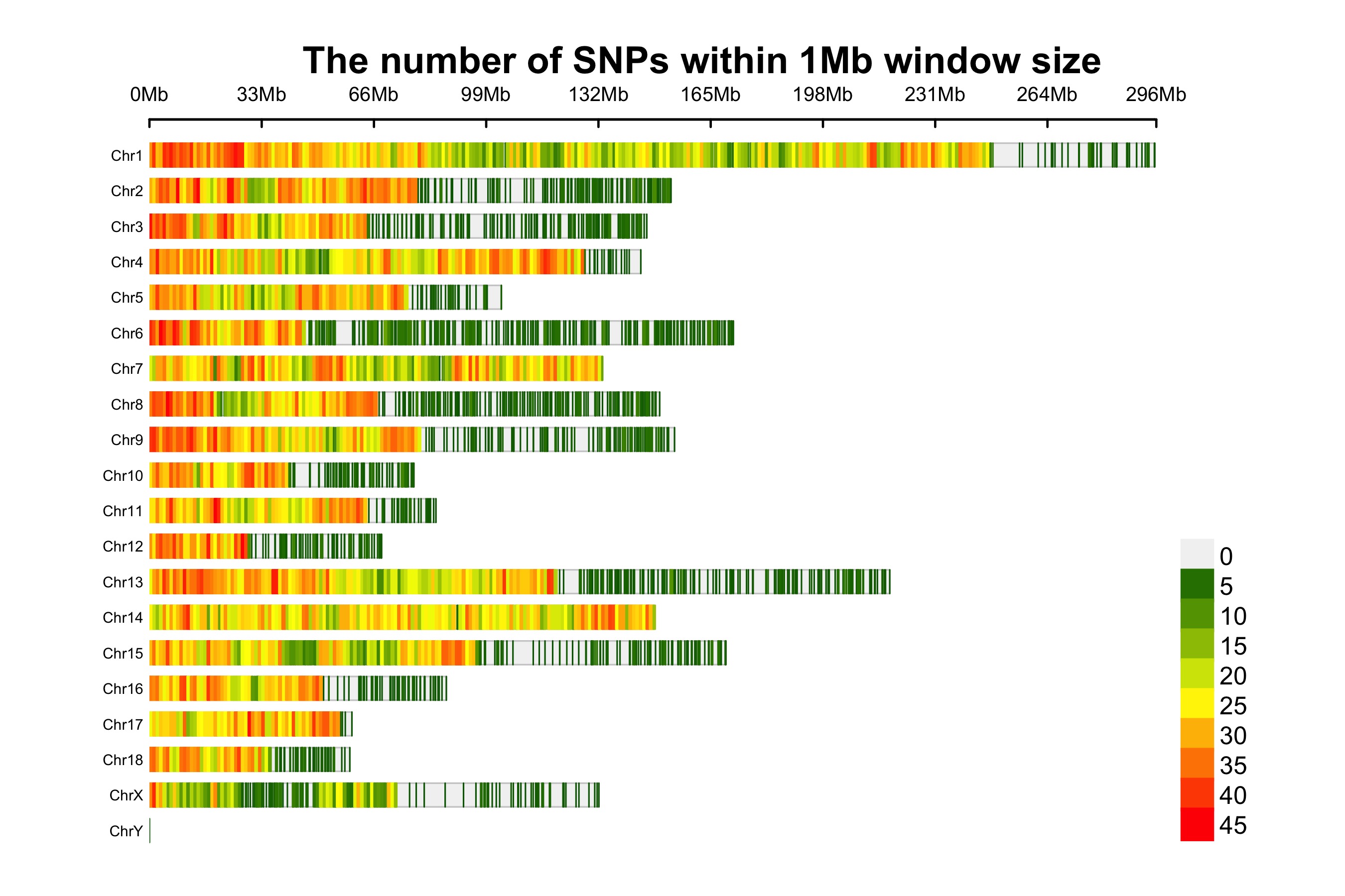
> CMplot(pig60K,type="p",plot.type="c",chr.labels=paste("Chr",c(1:18,"X","Y"),sep=""),r=0.4,cir.axis=TRUE,
outward=FALSE,cir.axis.col="black",cir.chr.h=1.3,chr.den.col="black",file="jpg",
file.name=NULL,dpi=300,file.output=TRUE,verbose=TRUE,width=10,height=10)
# to remove the grid line in circles, add parameter cir.axis.grid=FALSE# file.name: specify the output file name, the default is corresponding column name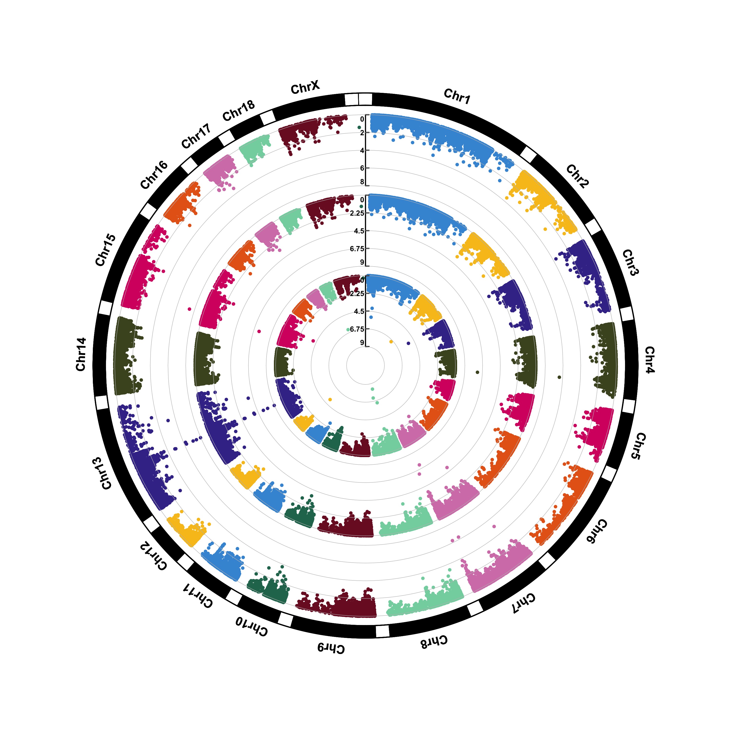
> CMplot(pig60K,type="p",plot.type="c",r=0.4,col=c("grey30","grey60"),chr.labels=paste("Chr",c(1:18,"X","Y"),sep=""),
threshold=c(1e-6,1e-4),cir.chr.h=1.5,amplify=TRUE,threshold.lty=c(1,2),threshold.col=c("red",
"blue"),signal.line=1,signal.col=c("red","green"),chr.den.col=c("darkgreen","yellow","red"),
bin.size=1e6,outward=FALSE,file="jpg",file.name=NULL,dpi=300,file.output=TRUE,verbose=TRUE,width=10,height=10)
#Note:1.ifsignal.line=NULL, thelinesthatcrossecircleswon't be added.2. if the length of parameter 'chr.den.col' is not equal to 1, SNP density that counts  the number of SNP within given size('bin.size') will be plotted around the circle.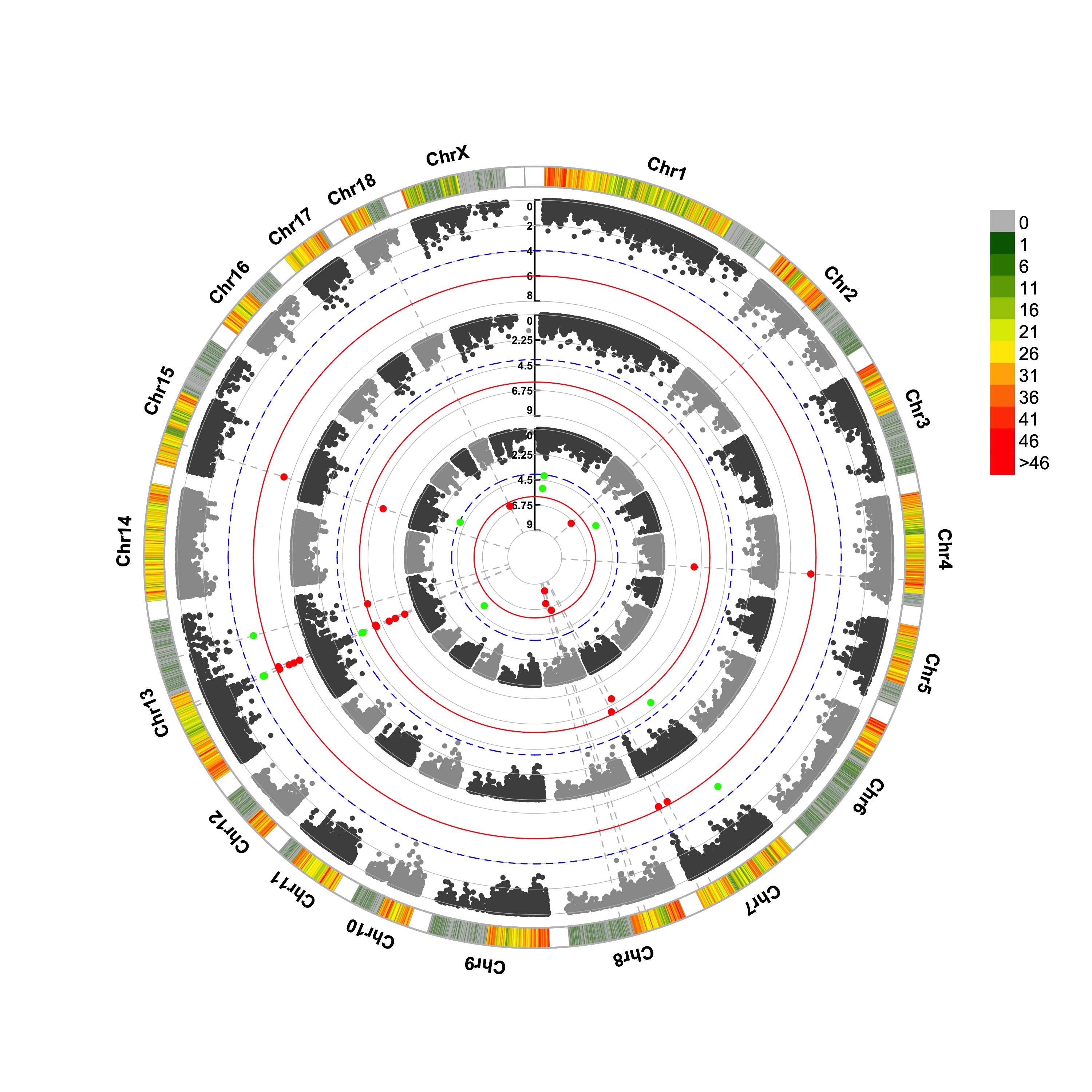
> CMplot(cattle50K,type="p",plot.type="c",LOG10=FALSE,outward=TRUE,col=matrix(c("#4DAF4A",NA,NA,"dodgerblue4",
"deepskyblue",NA,"dodgerblue1", "olivedrab3", "darkgoldenrod1"), nrow=3, byrow=TRUE),
chr.labels=paste("Chr",c(1:29),sep=""),threshold=NULL,r=1.2,cir.chr.h=1.5,axis.cex=1,
cir.band=1,file="jpg", file.name=NULL,dpi=300,chr.den.col="black",file.output=TRUE,verbose=TRUE,
width=10,height=10)
# parameter 'col' can be either vector or matrix, if a matrix, each trait can be plotted in different colors.# file.name: specify the output file name, the default is corresponding column name when setting ' file.name=NULL '
> CMplot(pig60K,type="p",plot.type="m",LOG10=TRUE,threshold=NULL,file="jpg",file.name=NULL,dpi=300,
file.output=TRUE,verbose=TRUE,width=14,height=6,chr.labels.angle=45)
# 'chr.labels.angle': adjust the angle of labels of x-axis (-90 < chr.labels.angle < 90).# file.name: specify the output file name, the default is corresponding column name when setting ' file.name=NULL '.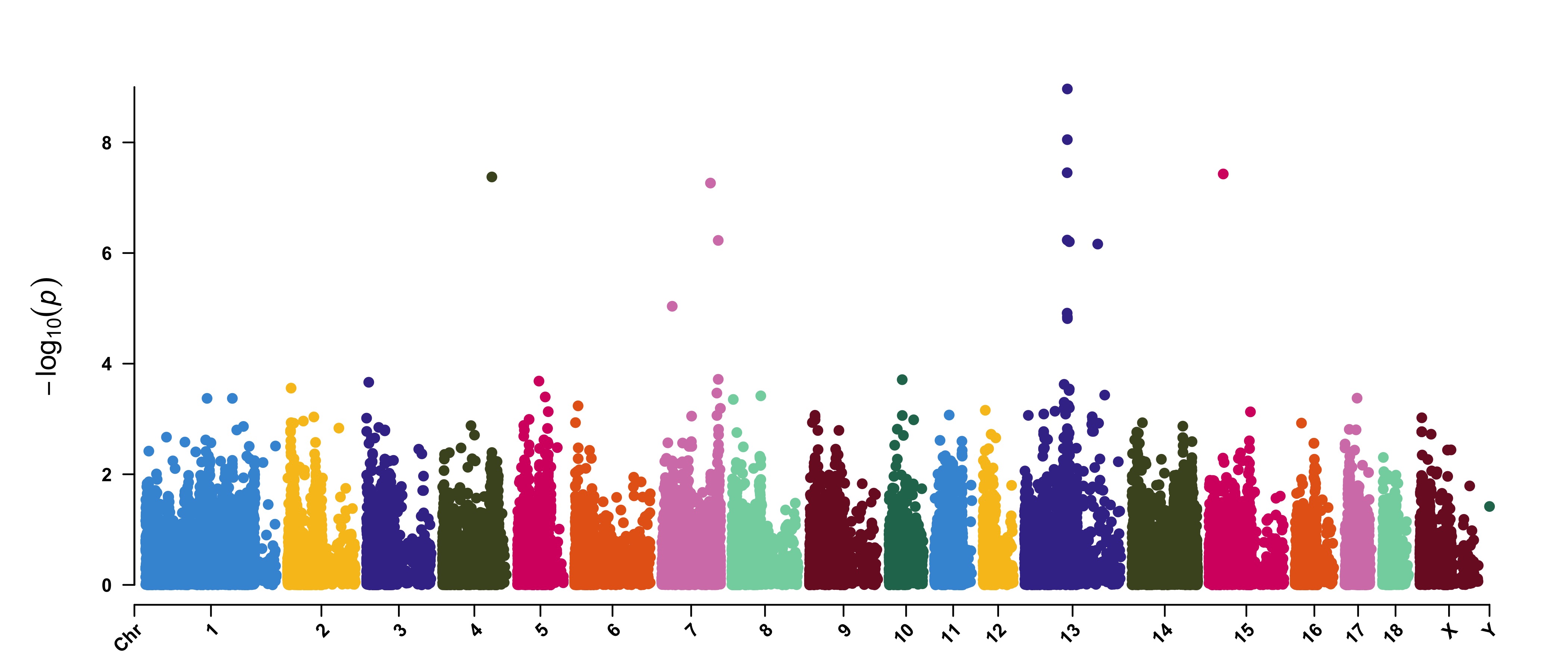
> CMplot(pig60K, plot.type="m", col=c("grey30","grey60"), LOG10=TRUE, ylim=c(2,12), threshold=c(1e-6,1e-4),
threshold.lty=c(1,2), threshold.lwd=c(1,1), threshold.col=c("black","grey"), amplify=TRUE,
chr.den.col=NULL, signal.col=c("red","green"), signal.cex=c(1.5,1.5),signal.pch=c(19,19),
file="jpg",file.name=NULL,dpi=300,file.output=TRUE,verbose=TRUE,width=14,height=6)
#Note: if the ylim is setted, then CMplot will only plot the points among this interval,# ylim can be vector or list, if it is a list, different traits can be assigned with# different range at y-axis.# 'threshold' can be set for different traits, for example: threshold=list(c(1e-6,1e-4), NULL, 1e-5),# each list contains a vector of thresholds for each trait, NULL means no threshold for corresponding trait. 
> CMplot(pig60K, plot.type="m", LOG10=TRUE, ylim=NULL, threshold=c(1e-6,1e-4),threshold.lty=c(1,2),
threshold.lwd=c(1,1), threshold.col=c("black","grey"), amplify=TRUE,bin.size=1e6,
chr.den.col=c("darkgreen", "yellow", "red"),signal.col=c("red","green"),signal.cex=c(1.5,1.5),
signal.pch=c(19,19),file="jpg",file.name=NULL,dpi=300,file.output=TRUE,verbose=TRUE,
width=14,height=6)
# Note: if the length of parameter 'chr.den.col' is bigger than 1, SNP density that counts# the number of SNP within given size('bin.size') will be plotted. # file.name: specify the output file name, the default is corresponding column name when setting file.name=NULL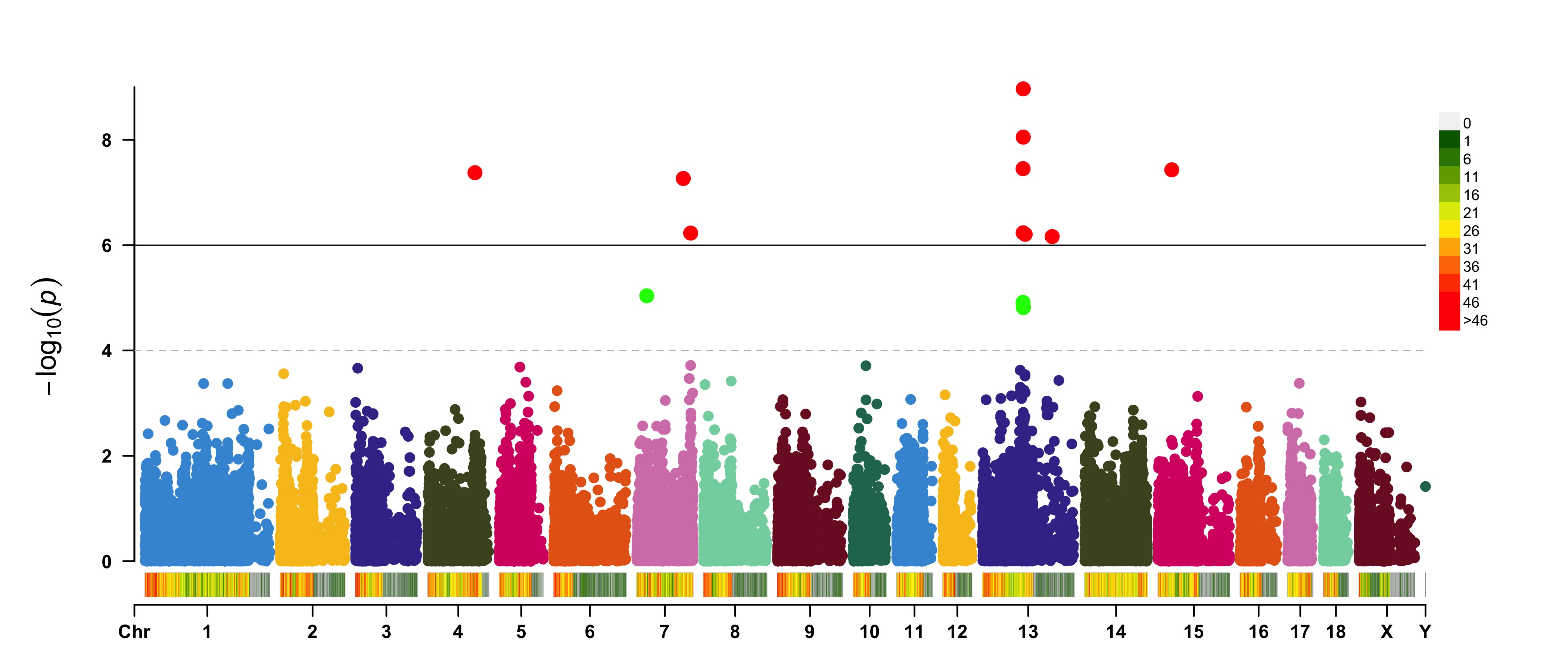
>signal<-pig60K$Position[which.min(pig60K$trait2)]
>SNPs<-pig60K$SNP[pig60K$Chromosome==13&pig60K$Position<(signal+1000000)&pig60K$Position>(signal-1000000)]
> CMplot(pig60K, plot.type="m",LOG10=TRUE,col=c("grey30","grey60"),highlight=SNPs,
highlight.col="green",highlight.cex=1,highlight.pch=19,file="jpg",file.name=NULL,
chr.border=TRUE,dpi=300,file.output=TRUE,verbose=TRUE,width=14,height=6)
# Note:# 'highlight' could be vector or list, if it is a vector, all traits will use the same highlighted SNPs index, # if it is a list, the length of the list should equal to the number of traits.# highlight.col, highlight.cex, highlight.pch can be value or vector, if its length equals to the length of highlighted SNPs,# each SNPs have its special colour, size and shape.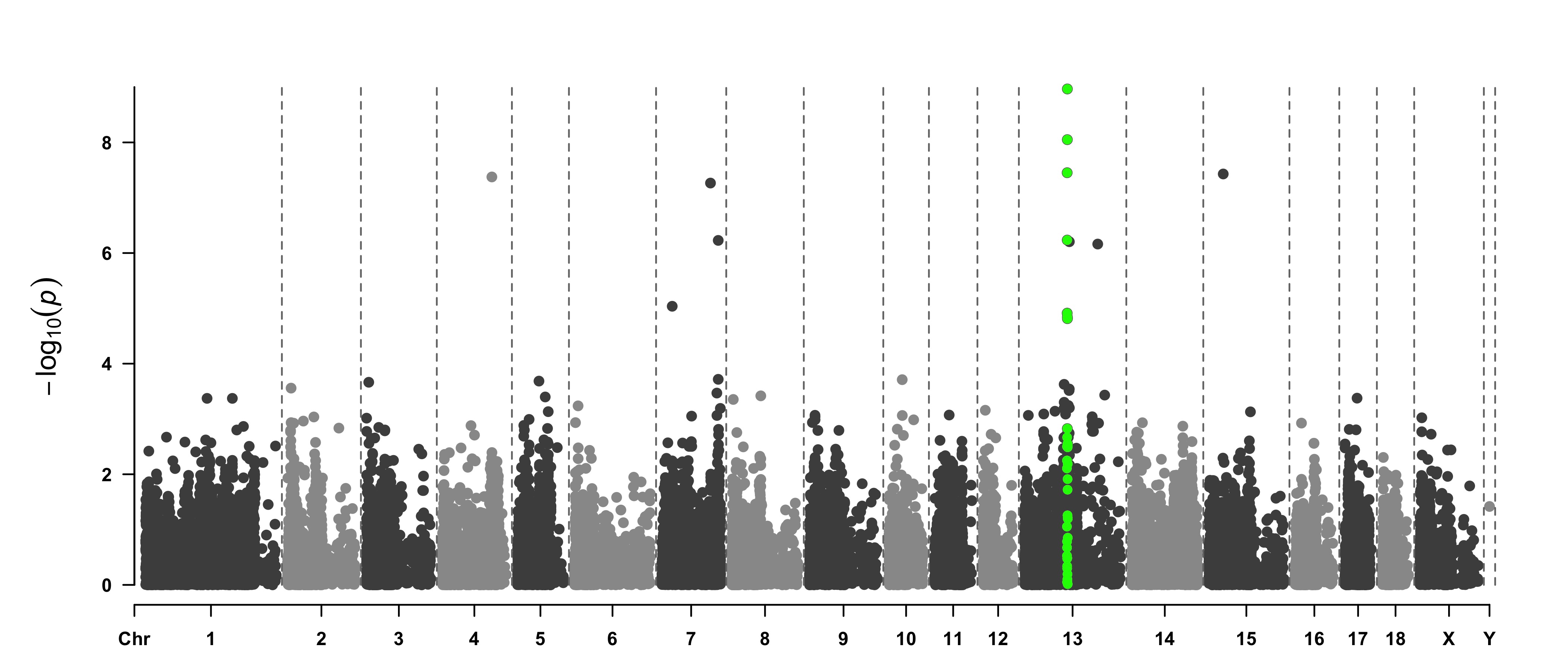
>SNPs<-pig60K[pig60K$trait2<1e-4, 1]
> CMplot(pig60K,type="h",plot.type="m",LOG10=TRUE,highlight=SNPs,highlight.type="p",
highlight.col=NULL,highlight.cex=1.2,highlight.pch=19,file="jpg",file.name=NULL,
dpi=300,file.output=TRUE,verbose=TRUE,width=14,height=6,band=0.6)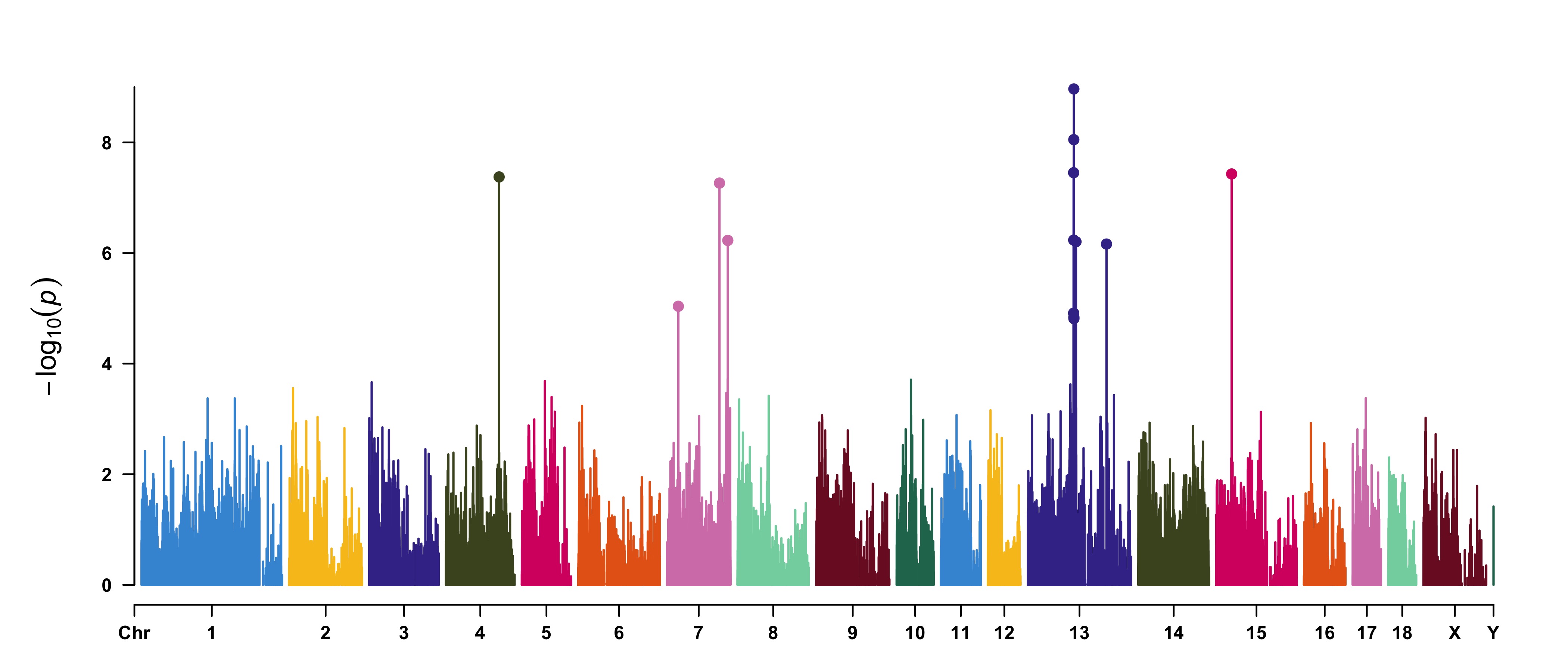
>SNPs<-pig60K[pig60K$trait2<1e-4, 1]
> CMplot(pig60K,type="p",plot.type="m",LOG10=TRUE,highlight=SNPs,highlight.type="h",
col=c("grey30","grey60"),highlight.col="darkgreen",highlight.cex=1.2,highlight.pch=19,
file="jpg",dpi=300,file.output=TRUE,verbose=TRUE,width=14,height=6)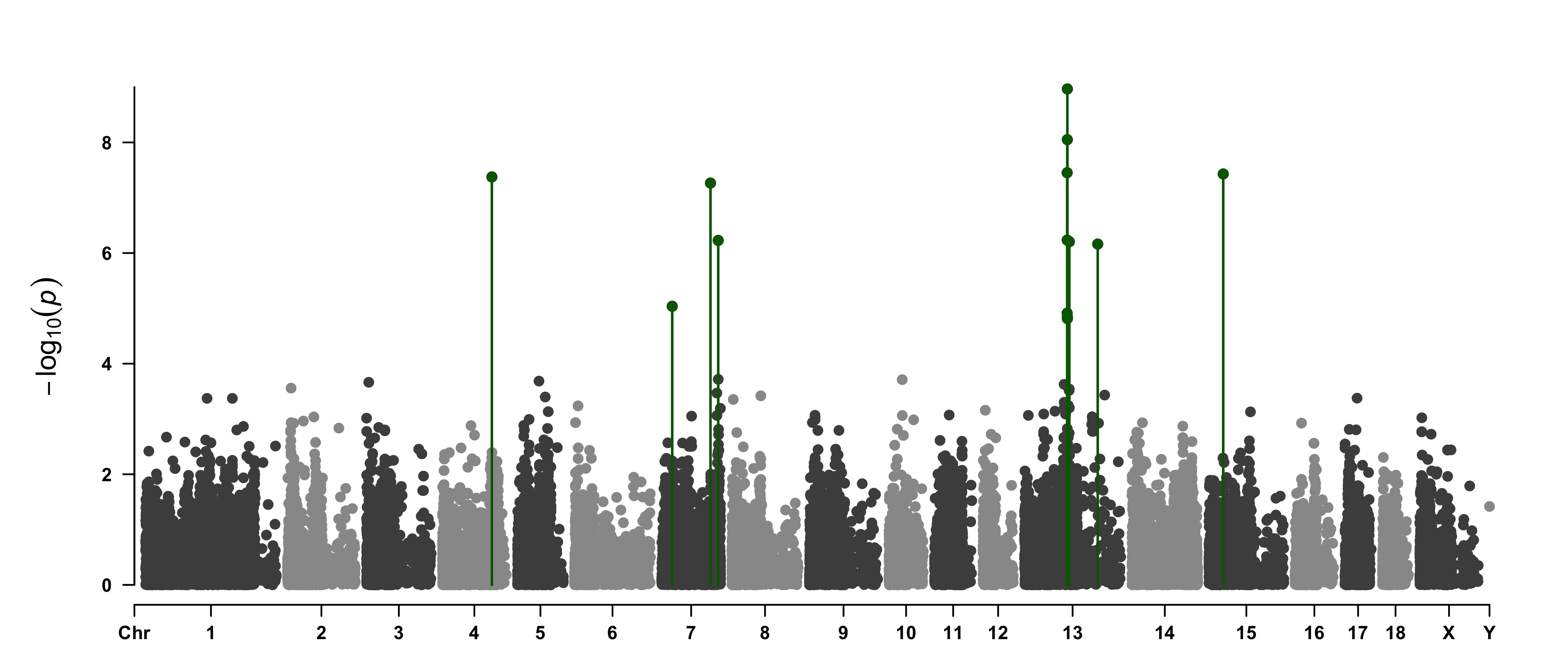
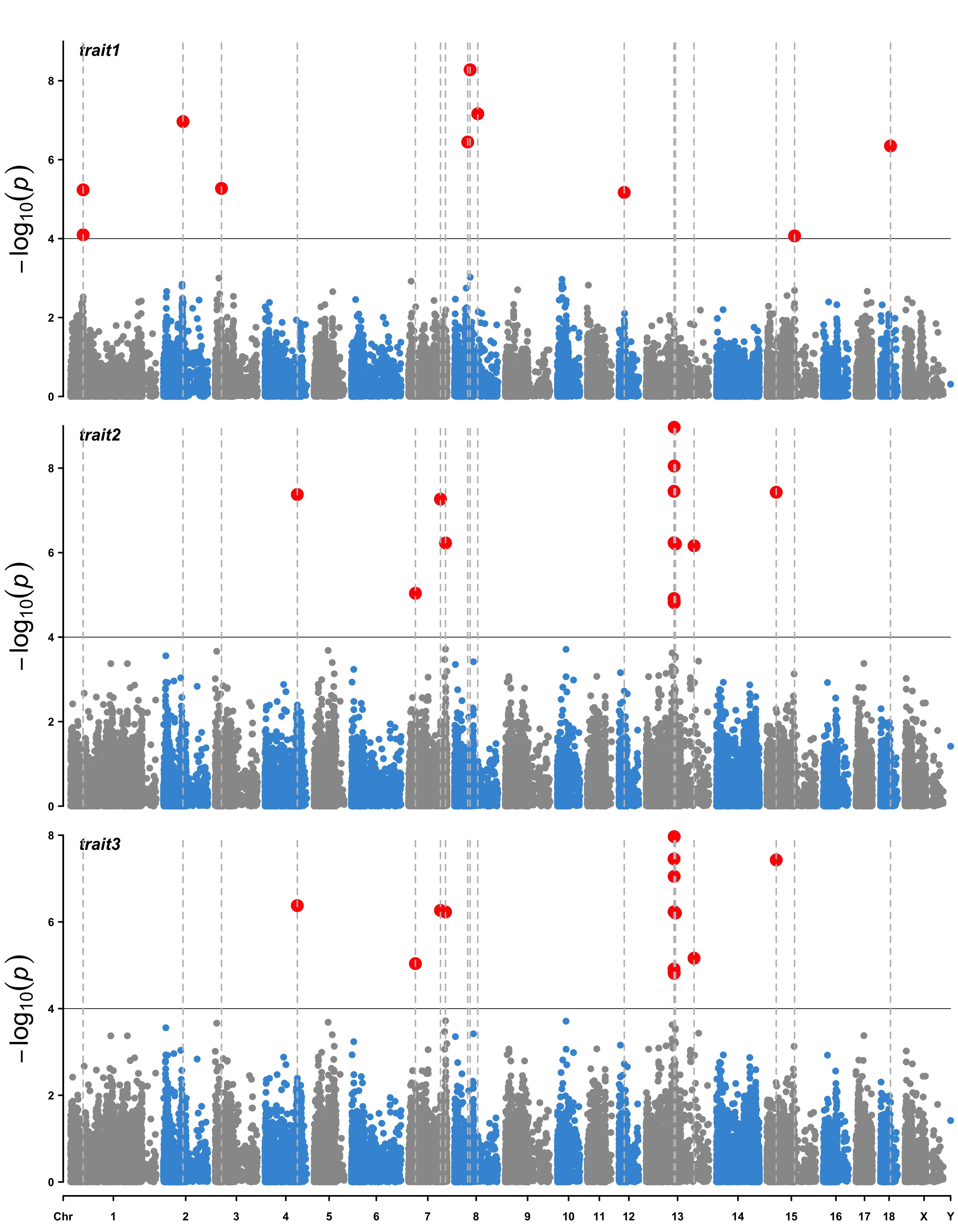
>SNPs<-pig60K[
pig60K$trait1<1e-4|pig60K$trait2<1e-4|pig60K$trait3<1e-4, 1]
> CMplot(pig60K,type="p",plot.type="m",LOG10=TRUE,highlight=SNPs,highlight.type="l",
threshold=1e-4,threshold.col="black",threshold.lty=1,col=c("grey60","#4197d8"),
signal.cex=1.2, signal.col="red", highlight.col="grey",highlight.cex=0.7,
file="jpg",dpi=300,file.output=TRUE,verbose=TRUE,multracks=TRUE)
> CMplot(pig60K[pig60K$Chromosome==13, ], plot.type="m",LOG10=TRUE,col=c("grey60"),highlight=SNPs,
highlight.col="green",highlight.cex=1,highlight.pch=19,file="jpg",file.name=NULL, threshold=c(1e-6,1e-4),threshold.lty=c(1,2),threshold.lwd=c(1,2), width=9,height=6,
threshold.col=c("red","blue"),amplify=FALSE,dpi=300,file.output=TRUE,verbose=TRUE)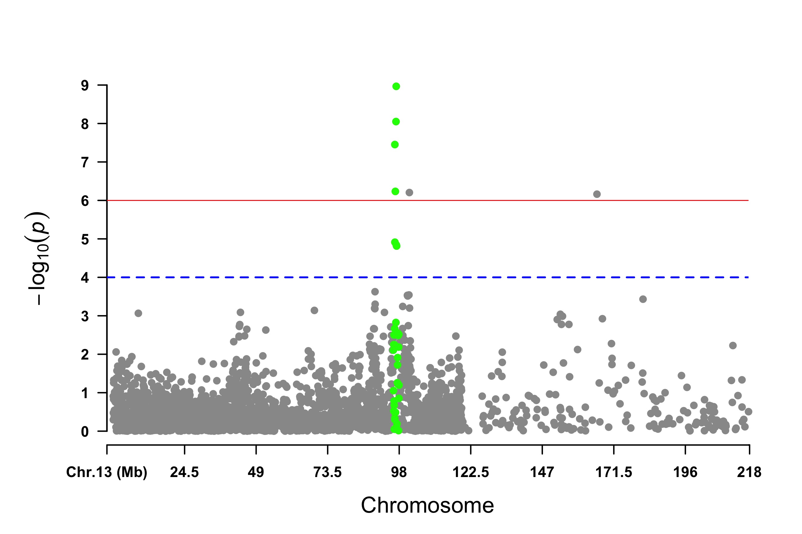
>SNPs<-pig60K[pig60K[,5] < (0.05/ nrow(pig60K)), 1]
>genes<- paste("GENE", 1:length(SNPs), sep="_")
> set.seed(666666)
> CMplot(pig60K[,c(1:3,5)], plot.type="m",LOG10=TRUE,col=c("grey30","grey60"),highlight=SNPs,
highlight.col=rep(c("green","blue"),length=length(SNPs)),highlight.cex=1, highlight.text=genes, highlight.text.col=rep("red",length(SNPs)),threshold=0.05/nrow(pig60K),threshold.lty=2, amplify=FALSE,file="jpg",file.name=NULL,dpi=300,file.output=TRUE,verbose=TRUE,width=14,height=6)
# Note:# 'highlight', 'highlight.text' could be vector or list, if it is a vector, all traits will # use the same highlighted SNPs index and text, if it is a list, the length of the list should equal to the number of traits.# the order of 'highlight.text' must be consistent with 'highlight'# highlight.text.cex: value or vecter, control the size of added text# highlight.text.font: value or vecter, control the font of added text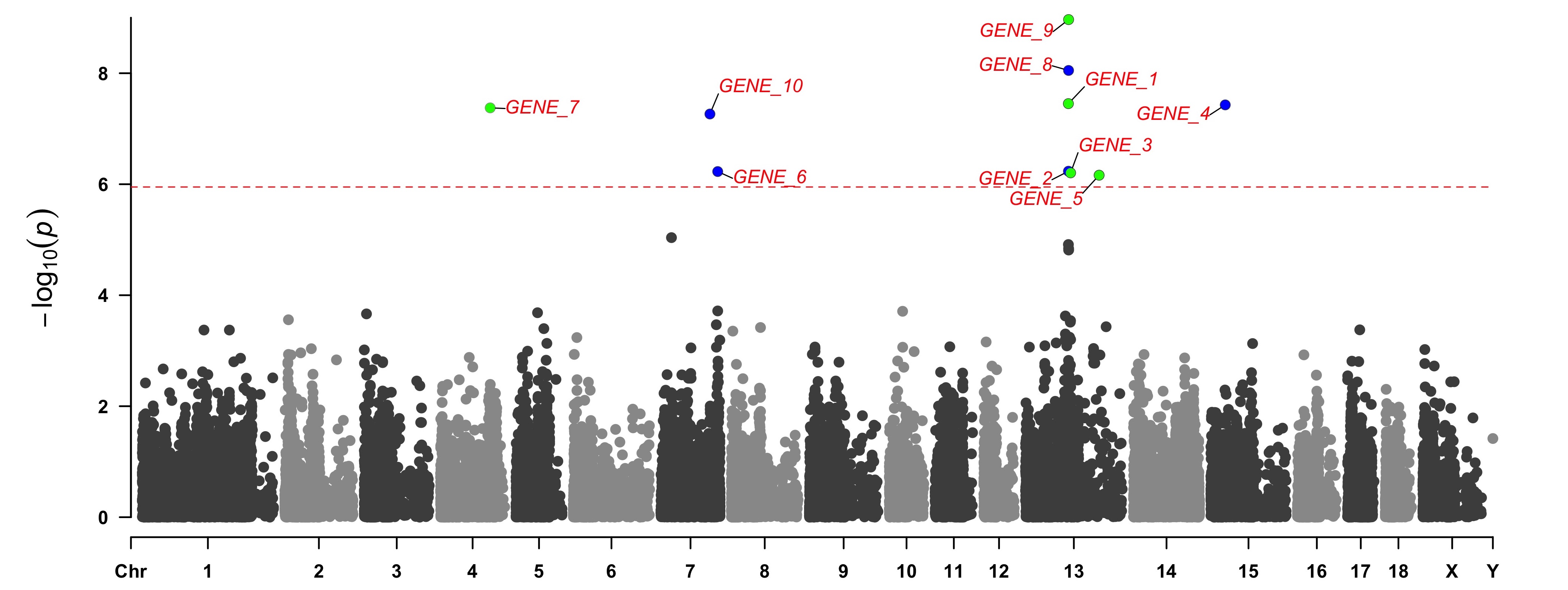
> CMplot(cattle50K, plot.type="m", band=0.5, LOG10=FALSE, ylab="SNP effect",threshold=0.015,
threshold.lty=2, threshold.lwd=1, threshold.col="red", amplify=TRUE, width=14,height=6,
signal.col=NULL, chr.den.col=NULL, file="jpg",file.name=NULL,dpi=300,file.output=TRUE,
verbose=TRUE,cex=0.8)
#Note: if signal.col=NULL, the significant SNPs will be plotted with original colors.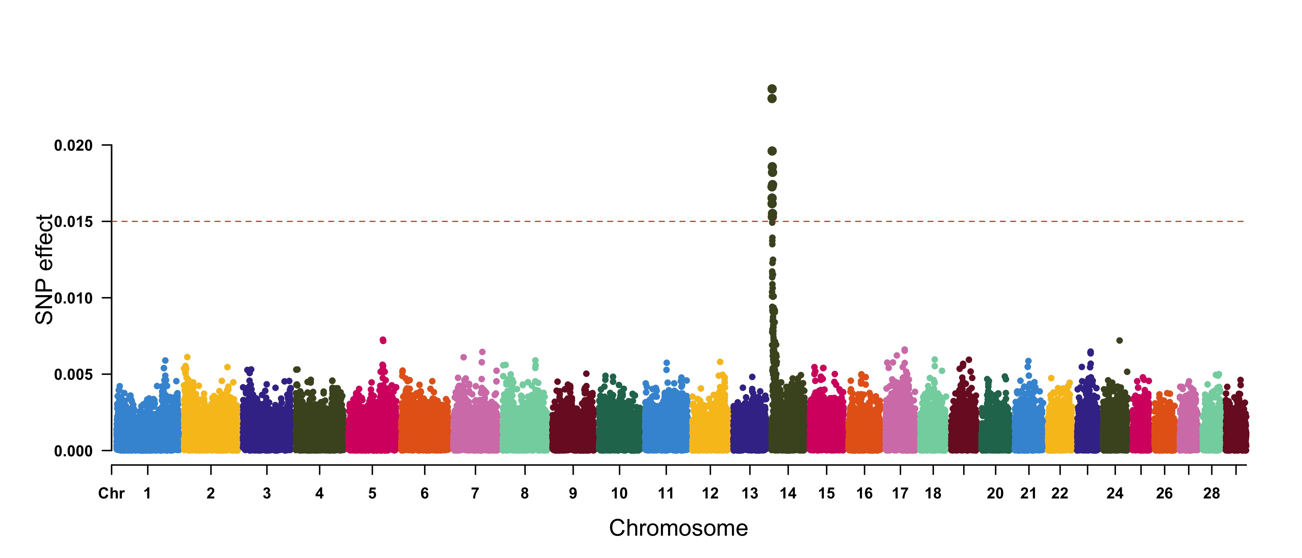
>cattle50K[,4:ncol(cattle50K)] <- apply(cattle50K[,4:ncol(cattle50K)], 2, function(x) x*sample(c(1,-1), length(x), rep=TRUE))
> CMplot(cattle50K, type="h",plot.type="m", band=0.5, LOG10=FALSE, ylab="SNP effect",ylim=c(-0.02,0.02),
threshold.lty=2, threshold.lwd=1, threshold.col="red", amplify=FALSE,cex=0.6,
chr.den.col=NULL, file="jpg",file.name=NULL,dpi=300,file.output=TRUE,verbose=TRUE)
#Note: Positive and negative values are acceptable.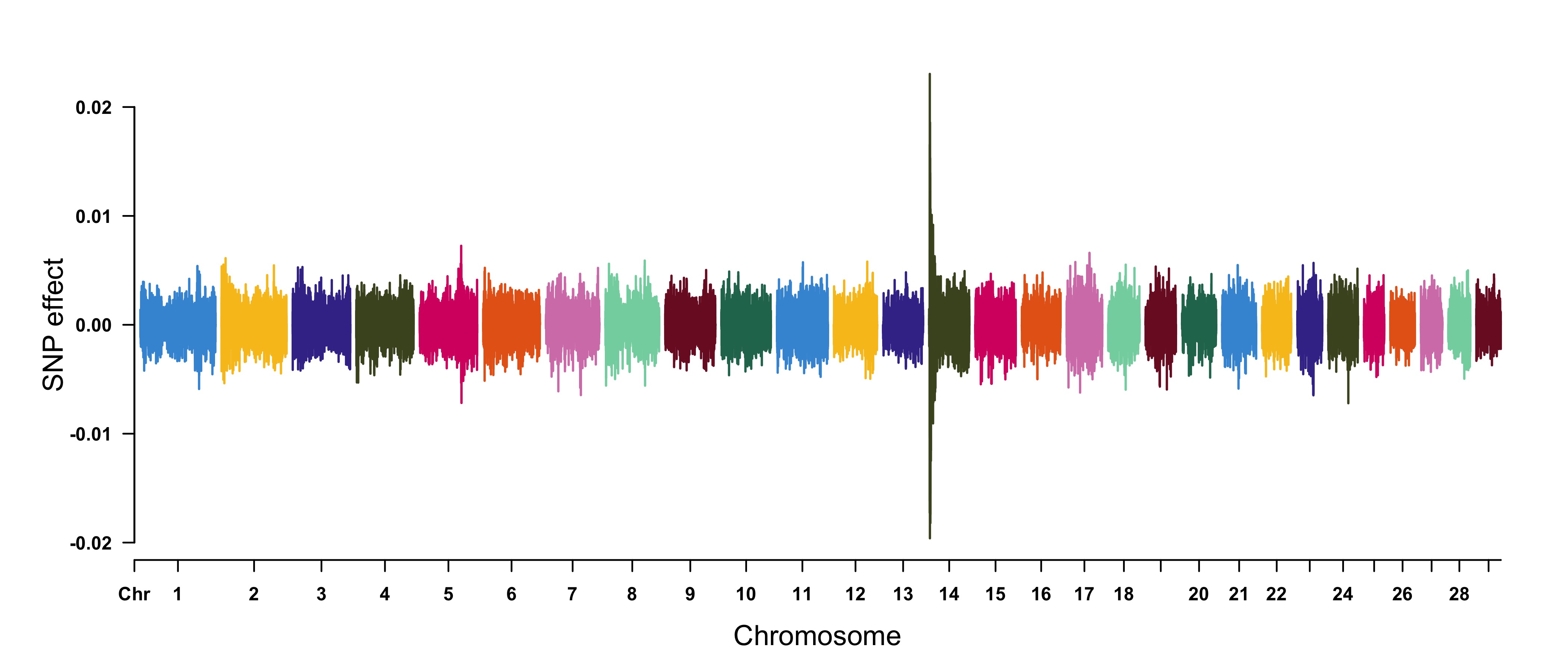
>SNPs<-list(
pig60K$SNP[pig60K$trait1<1e-6],
pig60K$SNP[pig60K$trait2<1e-6],
pig60K$SNP[pig60K$trait3<1e-6]
)
> CMplot(pig60K, plot.type="m",multracks=TRUE,threshold=c(1e-6,1e-4),threshold.lty=c(1,2), threshold.lwd=c(1,1), threshold.col=c("black","grey"), amplify=TRUE, signal.col=
c("red","green"), signal.cex=1, file="jpg",file.name=NULL,dpi=300,file.output=TRUE,
verbose=TRUE, highlight=SNPs, highlight.text=SNPs, highlight.text.cex=1.4)
#Note: if you are not supposed to change the color of signal, # please set signal.col=NULL and highlight.col=NULL.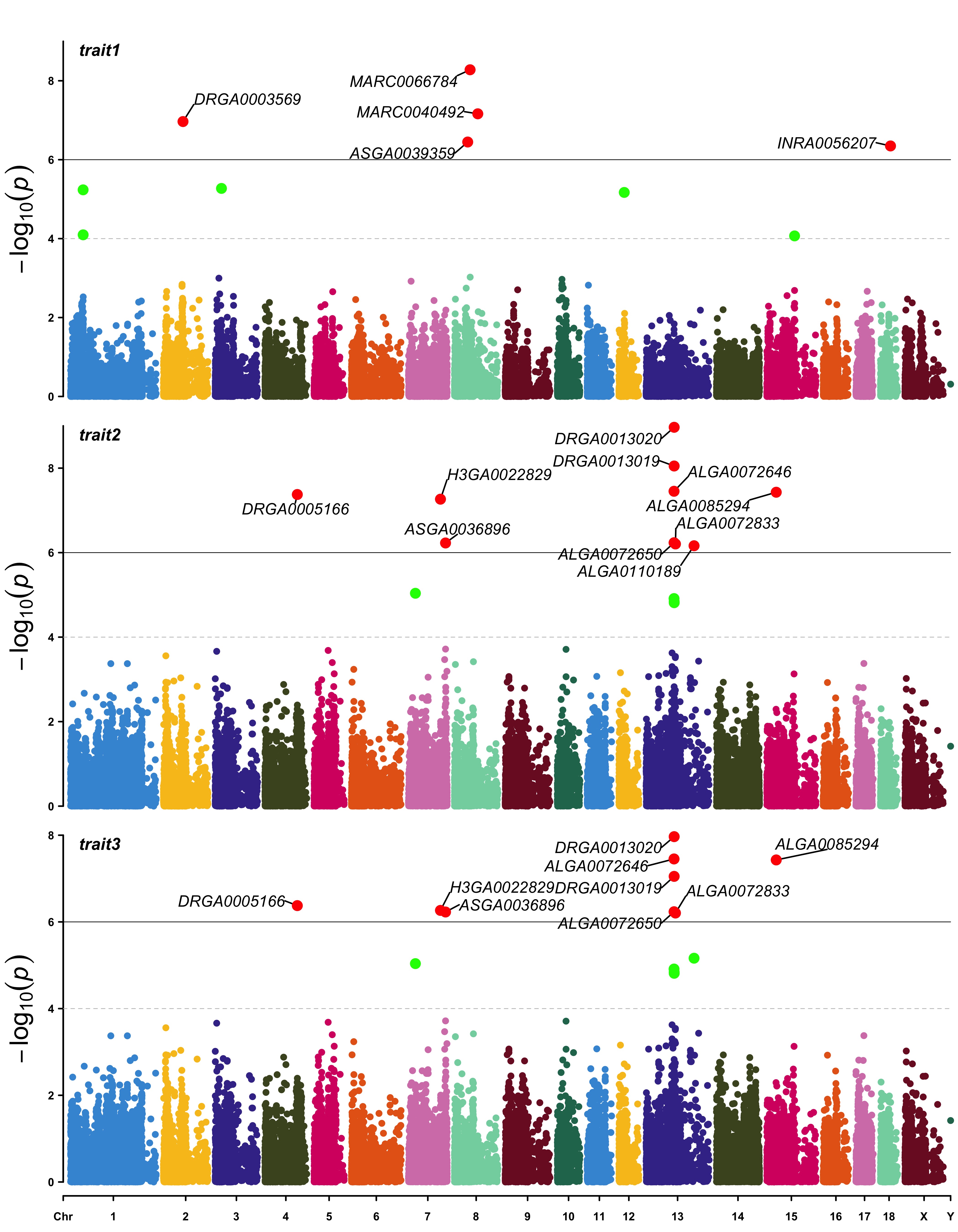
> CMplot(pig60K, plot.type="m",multraits=TRUE,threshold=c(1e-6,1e-4),threshold.lty=c(1,2), threshold.lwd=c(1,1), threshold.col=c("black","grey"), amplify=TRUE,bin.size=1e6,
chr.den.col=c("darkgreen", "yellow", "red"), signal.col=c("red","green"),
signal.cex=1, file="jpg",file.name=NULL,dpi=300,file.output=TRUE,verbose=TRUE,
points.alpha=100,legend.ncol=1, legend.pos="left")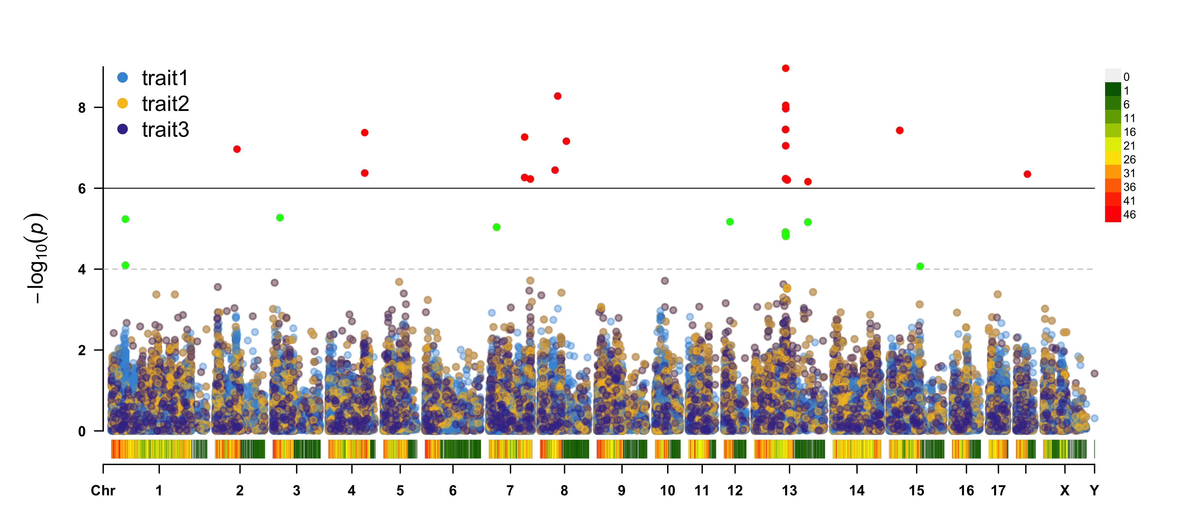
>CMplot(pig60K, plot.type="m",col="grey",multraits=TRUE,threshold=1e-4,threshold.lty=1, threshold.lwd=c(1,1), threshold.col=c("black","grey"),amplify=TRUE,
chr.den.col=NULL, signal.col=c("red","green","blue"),signal.cex=1, file="jpg",file.name=NULL,dpi=300,file.output=TRUE,verbose=TRUE,
points.alpha=225,legend.ncol=3, legend.pos="middle")
# note: length of 'col' should be equal to 1 for this case.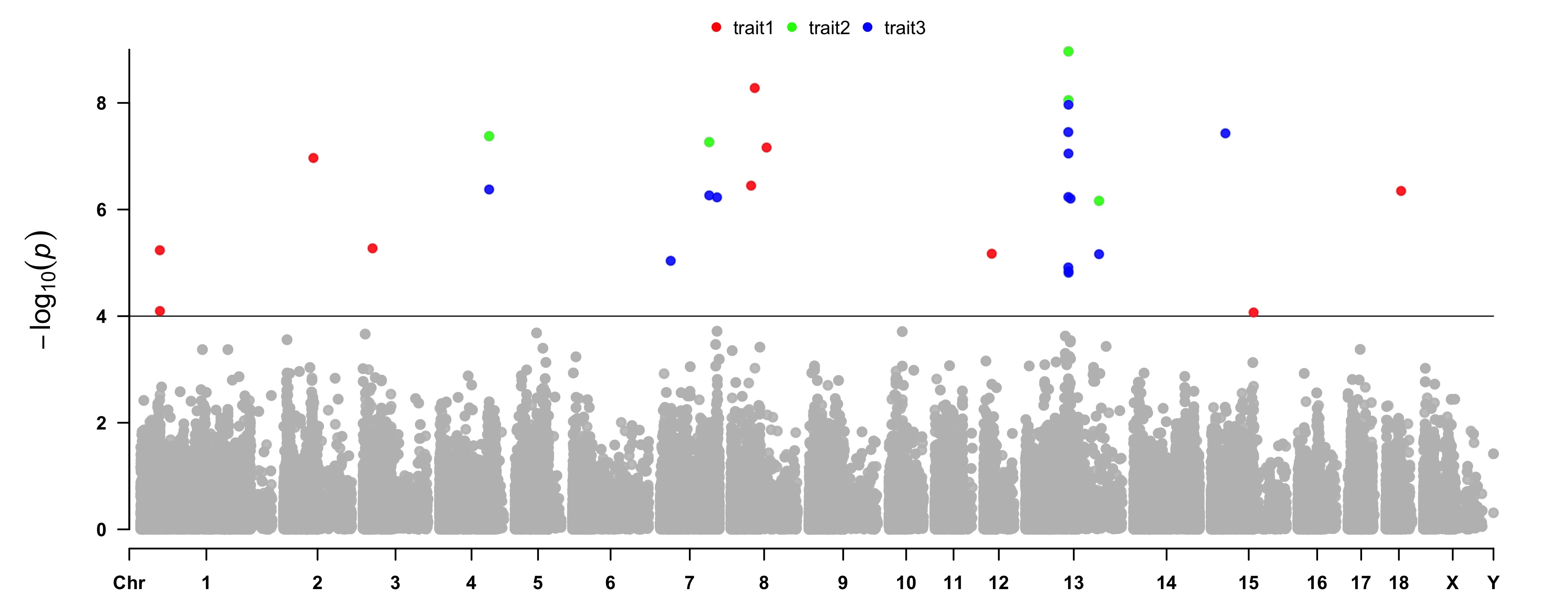 ---
---
> CMplot(pig60K,plot.type="q",box=FALSE,file="jpg",file.name=NULL,dpi=300,
conf.int=TRUE,conf.int.col=NULL,threshold.col="red",threshold.lty=2,
file.output=TRUE,verbose=TRUE,width=5,height=5)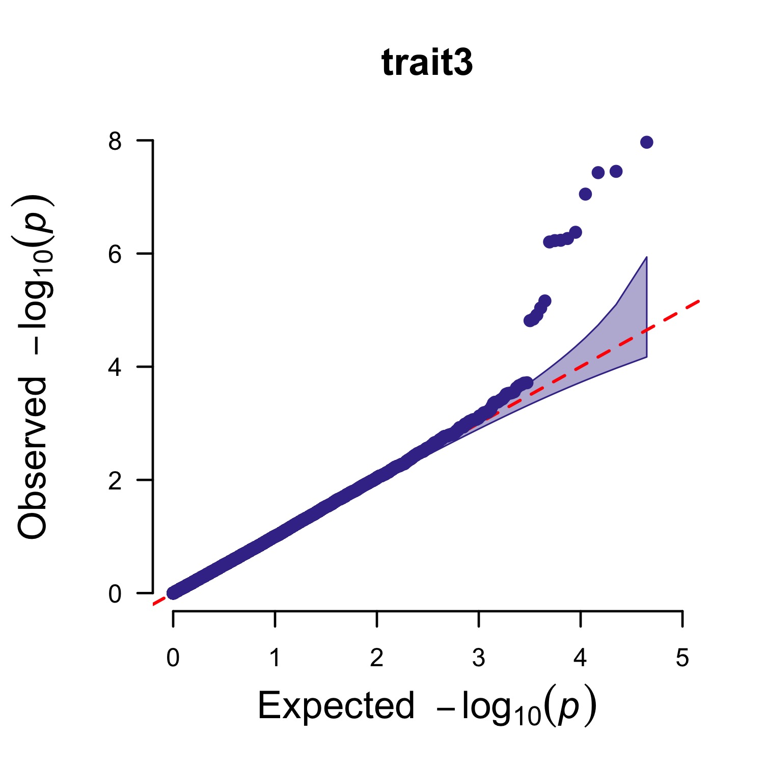
>pig60K$trait1[sample(1:nrow(pig60K), round(nrow(pig60K)*0.80))] <-NA>pig60K$trait2[sample(1:nrow(pig60K), round(nrow(pig60K)*0.25))] <-NA> CMplot(pig60K,plot.type="q",col=c("dodgerblue1", "olivedrab3", "darkgoldenrod1"),multracks=TRUE,
threshold=1e-6,ylab.pos=2,signal.pch=c(19,6,4),signal.cex=1.2,signal.col="red",
conf.int=TRUE,box=FALSE,axis.cex=2,file="jpg",file.name=NULL,dpi=300,file.output=TRUE,
verbose=TRUE,ylim=c(0,8),width=5,height=5)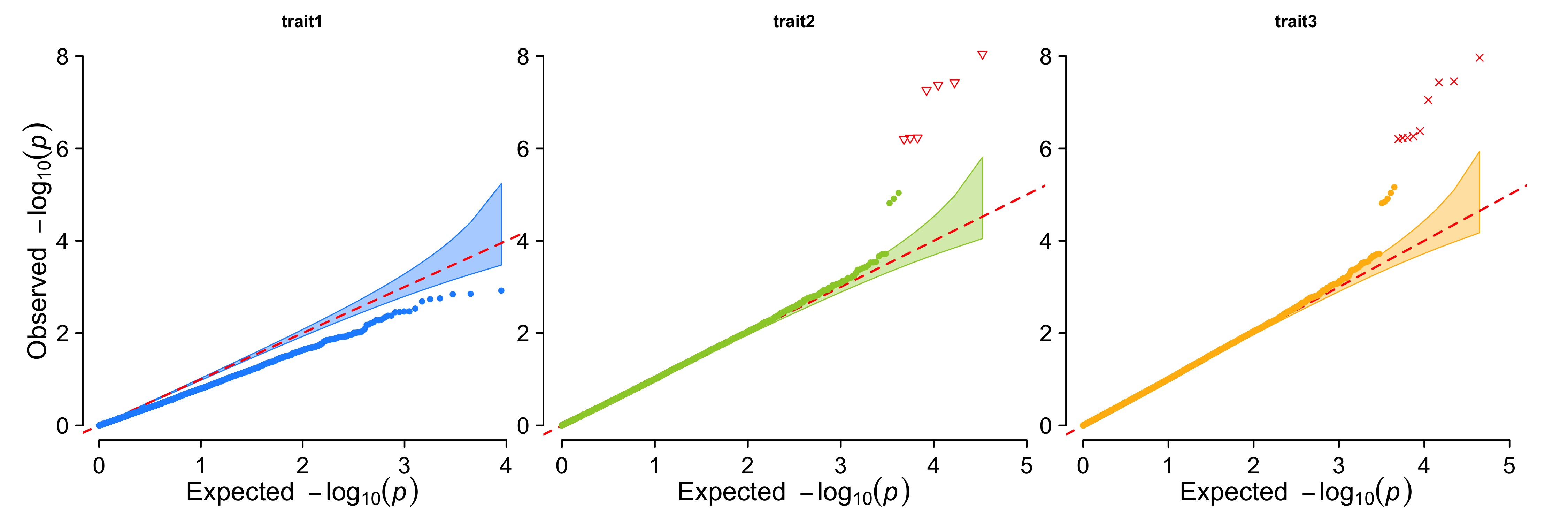
> CMplot(pig60K,plot.type="q",col=c("dodgerblue1", "olivedrab3", "darkgoldenrod1"),multraits=TRUE,
threshold=1e-6,ylab.pos=2,signal.pch=c(19,6,4),signal.cex=1.2,signal.col="red",
conf.int=TRUE,box=FALSE,axis.cex=1,file="jpg",file.name=NULL,dpi=300,file.output=TRUE,
verbose=TRUE,ylim=c(0,8),width=5,height=5)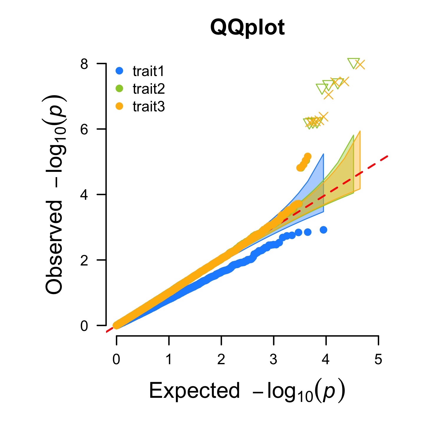
Questions, suggestions, and bug reports are welcome and appreciated.
- Author: Lilin Yin
- Contact:ylilin@163.com
- QQ group: 166305848
- Institution:Huazhong agricultural university