Chplot - Arbitrary functions plotting and computations

Chplot is a Python >= 3.9 module to plot any arbitrary mathematical expressions as well as data series from files, and compute its derivatives and integrals, where it equals zero, linear and non-linear regressions, and much more !

Installation

chplot is available on Pypi, and You can install it with the command:

python -m pip install chplot

You can also install it by cloning this repo and installing it directly:

git clone https://github.com/charon25/Chplot.git
cd Chplot
python -m pip install .

To check it is properly installed, just run and check it outputs the current version:

python -m chplot --version

This module requires the following third-party modules:

• matplotlib >= 3.6.1
• mpmath >= 1.2.1
• numpy >= 1.23.4
• scipy >= 1.9.3
• shunting_yard >= 1.0.12
• tqdm >= 4.64.1

Usage

In the rest of this README, the term "expression" will refer to any mathematical expression, possibly with one variable (by default x but can be changed).

From a CLI

This module is primarly intended to be used in the command-line. To do this, use the following command:

python -m chplot [expression1, [expression2, ...]] [additional-parameters...]

Where all the additional parameters are documented in the CLI options section. Note that there can be no expression, as data can come from other sources.

A lot of examples are given in the Examples section.

Important note

You need to surround any expression with double quotes (") if it contains a space (). Furthermore, due to the working of the argparse Python module and the majority of shells, you may have to surround any expression with double quotes (") if it contains a caret (^). Finally, if it starts with a dash (-) you may also need to add a space () or a 0 before it. For instance, you need to write " -x" or "0-x" to get the function f(x) = -x and "x^2" (instead of just x^2) to get the square function.

From Python code

The chplot module can also be used from another program. Code snippets:

# Use this to use the built-in PlotParameters classimportchplotparameters=chplot.PlotParameters()
chplot.plot(parameters)

# Use this to use another object and set default valuesimportchplotparameters= ... # any objectchplot.set_default_values(parameters) # add any missing field with its default valuechplot.plot(parameters)

All the PlotParameters arguments are summarized in the CLI options section.

CLI options

No option is mandatory.

CLI options	PlotParameters class equivalent	Expected arguments	Effect
$\emptyset$	expressions: list[str]	Any number of expressions (including none of them) or filepaths	The expressions of the mathematical functions to plot and do computations on. If using the CLI, filepaths can also be provided, and There can by none of them.
-v --variable	variable: str	One string	The variable going of the horizontal axis. Can be more than one character. Note that the variable will override any constant of function with the same name. Defaults to x.
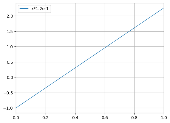
--no-sn	disable_scientific_notation: bool	$\emptyset$	Disable the automatic conversion of scientific notation in every expression (e.g. 1.24e-1 to 1.24*10^(-1)). Defaults to False.
-n --n-points	n_points: int	One positive integer (excluding zero)	The number of points on the horizontal axis for the plotting of the expressions. Defaults to 10001.
-i --integers	is_integer: bool	$\emptyset$	Forces the points where the expressions are computed to be integers between the specified limits. The number of points will not exceed what is specified with the -n parameter. Defaults to False.
-x --x-lim	x_lim: tuple[float|str|None, float|str|None]	Two expressions	The horizontal axis bounds (inclusive) where the expression are computed. First argument is the min, second is the max. Any expression (such as 2pi or 1+exp(2)) is valid. It is also the graph default horizontal axis, but they can be automatically adjusted to accomodate the plotted data. Defaults to 0 1.
-xlog --xlog	is_x_log: bool	$\emptyset$	Forces a logarithmic scale on the horizontal axis. If some horizontal axis bounds are negative, will modify them. Defaults to False.
-y --y-lim	y_lim: tuple[float|str|None, float|str|None]	Two expressions	The vertical axis bounds (inclusive) of the graph. First argument is the min, second is the max. Any expression (such as 2pi or 1+exp(2)) is valid. If not specified, will use matplotlib default ones to accomodate all data. Will restrict the graph to them is specified.
-z --y-zero	must_contain_zero: bool	$\emptyset$	Forces the vertical axis to contain zero. Defaults to False.
-ylog --ylog	is_y_log: bool	$\emptyset$	Forces a logarithmic scale on the vertical axis. If some vertical axis bounds are negative, will modify them. Defaults to False.
-xl --x-label	x_label: str	One string	Label of the horizontal axis. Defaults to nothing.
-yl --y-label	y_label: str	One string	Label of the vertical axis. Defaults to nothing.
-t --title	title: str	One string	Title of the graph. Defaults to nothing.
-rl --remove-legend	remove_legend: bool	$\emptyset$	Removes the graph legend. Defaults to False.
--no-plot	no_plot: bool	$\emptyset$	Does not show the plot. However, does not prevent saving the figure. Defaults to False.
-dis --discontinuous	markersize: int|None	One optional positive integer (excluding zero)	Transforms the style of the graph from a continuous line to discrete points with the specified radius. If present without a value, will defaults to a radius of 1. If the --integer parameter is also present, will still affect the points radius.
--square	square_graph: bool	$\emptyset$	Forces the graph to be a square (aspect ratio of 1). Defaults to False.
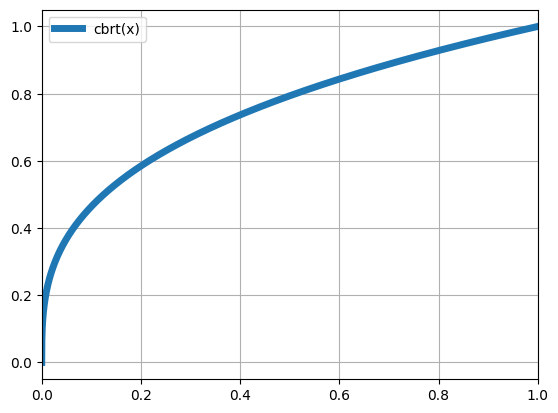
-lw --line-width	line_width: float	One positive float (excluding zero)	Width of the plotted functions. Will not affect regressions. Defaults to 1.5 (matplotlib defaut).
-c --constants	constants: list[str]	One string or more, either a filepath or of the forme <name>=<expression>	Adds constants which may be used by any other expressions (including axis bounds). They must either be of the form <name>=<expression> (eg a=4sin(pi/4)) or be filepath containing lines respecting this format. Note that filepaths are only accepted in the CLI. May override already existing constants and functions. If a constant refers to another one, it should be defined after. Defaults to nothing.
-f --files	data_files: list[str]	One or more filepaths	Adds data contained in CSV files as new functions to the graph. See the CSV files format section for more details. Defaults to nothing.
-s --save-graph	save_figure_path: str	One filepath	Saves the graph at the specified path. If not included, will not save the figure (default behavior).
-d --save-data	save_data_path: str	One filepath	Saves the graph data (x and y values) at the specified path in CSV format. If not included, will not save the data (default behavior).
-p --python-files	python_files: list[str]	One or more filepaths	Adds functions contained in Python files. See the Additional Python function format section for more details. Defaults to nothing.
--zeros	zeros_file: str|None	One optional filepath	Computes where the expressions equal zero. If not included, will not compute it (default behavior), else if included without argument, prints the results to the console, else writes it to the given file.
-int --integral	integral_file: str|None	One optional filepath	Computes the integral of all functions on the entire interval where it is plotted. Note that it does not add the antideritive of the functions to the graph, but only computes the area under them on their definition interval. If not included, will not compute it (default behavior), else if included without argument, prints the results to the console, else writes it to the given file.
-deriv --derivative	derivation_orders: list[int]	At least one positive integer (excluding zero)	Computes and adds to the graph the derivative of the specified orders of every other function. Note that the higher the order, the more inaccuracy and unstability it has. Furthermore, the derivative computation will shave off a few points on each side, so the derivatives are defined on a smaller interval.
-reg --regression	regression_expression: str	One expression	Computes the coefficients of the given regression to get the best fit to every other function. The regression parameters should have the form _rX where X is any string made of digits, letters and underscores and starting with a letter (eg _ra0). The regressions will also be added in the final graph. When using the CLI, the expression can also be one of a few default keywords (listed in Regression default keywords).

Options synergies

Every option that computes something based on the functions will act on every function defined before it applies. The order of application is the following (each item applies to all the previous ones):

• Base expressions & file data
• Regressions
• Derivations
• Integrals & zeros

For instance, this means every regression will also be derivated, and every derivative will be integrated.

CSV files format

The --file option will accept any CSV file respecting those rules:

• the column delimiter is eitehr a comma (,), a semicolon (;), a space () or a tabulation (\t) ;
• the decimal separator is either a dot (.) or a comma (,) if the column delimiter is something else (for countries and language using them, such as French or German) ;
• text entry containing the column delimiter must be surrounded by double quotes (") ;
• to have double quotes (") in a text entry, just double them ("").

The first column will be considered the horizontal axis data for the entire file. Each subsequent column will be a new function. They might all be of different lengths, and some value may be missing. Any missing value in the first column will ignore the whole line.

The first non numerical line will be used as label for the functions.

Examples

The file

x,"First y","Second ""y""",ThirdY,EmptyColumn0,0,,0,1,10,100,,2,20,,2000,3,30,300,3000,4,40,400,,

Will result in the following functions (represented as (x,y) couples):

• First y: (0, 0), (1, 10), (2, 20), (3, 30), (4, 40)
• Second "y": (1, 100), (3, 300), (4, 400)
• ThirdY: (0, 0), (2, 2000), (3, 3000)

Note that the last column does not have any values, so it won't be registered at all.

The file

x;y1;y20,0;1,0;2,10,3;1,2;2,50,6;1,55;2,1231;1,825;2,99

Will result in the following functions:

• y1: (0, 1), (0.3, 1.2), (0.6, 1.55), (1, 1.825)
• y2: (0, 2.1), (0.3, 2.5), (0.6, 2.123), (1, 2.99)

Regression default keywords

When using Chplot from the command line and using the --regression command, a keyword can be specified instead of an expression to get usual regression expression. Those keywords are listed below :

Keyword	Mathematical function	Equivalent expression
const constant	$f(x) = m$	_rm
lin linear	$f(x) = ax + b$	_ra * x + _rb
pN polyN polynomialN where $N \in \mathbb{N} $	$$f(x) = \sum_{i=0}^N a_i x^i$$	_ra0 _ra1 * x + _ra0 _ra2 * x^2 + _ra1 * x + _r0 ...
power	$f(x) = k x^\alpha$	_rk * x^_ralpha
powery	$f(x) = k x^\alpha + y_0$	_rk * x^_ralpha + r_y0
log	$f(x) = a \ln(x) + b$	_ra * ln(x) + _rb
exp	$f(x) = a \mathrm{e}^{bx}$	_ra * exp(x * _rb)
expy	$f(x) = a \mathrm{e}^{bx} + y_0$	_ra * exp(x * _rb) + _ry0

Note that poly0 is equivalent to constant and poly1 is equivalent to linear.

Additional Python function format

Chplot expression can accept functions usable in any expression directly from other Python files. Those file must respect those rules:

• they must be in the same directory as the console when using the CLI (and in the same directory as the python execution when using the code version [NOT TESTED]) ;
• all functions to add must be decorated with the @plottable decorator (importable with from chplot import plottable). The decorator must indicate how many arguments is expected by the function, either directly or with the arg_count keyword (i.e. @plottable(1) or @plottable(arg_count=2)) ;
• all functions must only accept int or float and must only return one value accepted by the float() built-in function of Python, such as, but not limited to, int, float or bool (if not, will be considered as the same as a raised Exception) ;
• to indicate an error in the computation (such as a division by zero or the square root of a negative number), the function can either raise an exception or return math.nan (or float('nan')). Note that an exception will completely stop the computation at that point while nan will be used in the rest of the expression, which may change the result slightly.

Everything other than those rules is allowed, such as importing other modules. The name of the Python function will be the same as the name used in the expression.

Examples

The Python file functions.py

fromchplotimportplottableimportmath@plottable(1)definc(x: float) ->float:
returnx+1@plottable(arg_count=2)definvradius(x: float, y: float) ->float:
ifx==y==0:
raiseZeroDivisionErrorreturn1/math.sqrt(x*x+y*y)
defdec(x: float) ->float:
returnx-1@plottabledefdouble(x: float) ->float:
returnx*2

Will define 2 new functions usable in expression: inc and invradius. dec does not have the decorator and will be ignored, and double does not indicate how many parameters it accepts, and therefore will also be ignored (but a warning will be logged).

This means, the following command is valid:

python -m chplot "inc(invradius(x, 5))" -x 1 inc(2) -p functions.py

Available functions

Chplot is bundled by default with more than 60 mathematical and physical constants and over 200 mathematical functions from the default math module, scipy.special, mpmath as well as custom made ones. They are all described in the following sections. The documentation of functions from math or the third-party modules can be found in their respective wikis: math, scipy.special, mpmath.

There are also the 5 base operations : +, -, *, /, ^.

Constants

nan and _ are valid constants that both evaluates to math.nan. They can be used to remove some points from the graph (for instance with the if or in functions, see below). inf is also a valid constant evaluating to math.inf.

Mathematical constants

chplot name	Name	Usual symbol	Exact value	chplot value
pi	Pi	$\pi$	$\pi$	$3.141\ 592\ 653\ 589\ 793$
tau	Tau	$\tau$	$2\pi$	$6.283\ 185\ 307\ 179\ 586$
e	Euler's number	$e$	$$\exp(1) = \sum_{n=0}^{+\infty} \frac{1}{n!}$$	$2.718\ 281\ 828\ 459\ 045$
ga em	Euler-Mascheroni's constant	$\gamma$	$$\lim_{n\to\infty} \left( \sum_{k=1}^n \left( \frac{1}{k}\right) - \log n \right)$$	$0.577\ 215\ 664\ 901\ 532 9$
phi	Golden ratio	$\phi$	$\frac{1}{2} (1 + \sqrt{5})$	$1.618\ 033\ 988\ 749\ 895$
sqrt2	Square root of 2	$\sqrt{2}$	$\sqrt{2}$	$1.414\ 213\ 562\ 373\ 095\ 1$
apery	Apery's constant		$$\zeta(3) = \sum_{n=1}^{+\infty} \frac{1}{n^3} $$	$1.202\ 056\ 903\ 159\ 594$
brun	Brun's constant	$B_2$	Sum of the reciprocal of the twin primes	$1.902\ 160\ 583\ 104$
catalan	Catalan's constant	$G$	$$\sum_{n=0}^{+\infty} \frac{(-1)^n}{(2n + 1)^2} $$	$0.915\ 965\ 594\ 177\ 219$
feigenbaumd	First Feigenbaum's constant	$\delta$		$4.669\ 201\ 609\ 102\ 990\ 67$
feigenbauma	Second Feigenbaum's constant	$\alpha$		$2.502\ 907\ 875\ 095\ 892\ 82$
glaisher	Glaisher-Khinkelin's constant	$A$	$$\lim_{n\to\infty} \frac{\Pi_{k=1}^{n} k^k}{n^{\frac{n^2}{2} + \frac{n}{2} + \frac{1}{12}}\cdot\mathrm{e}^{-\frac{n^2}{4}}}$$	$1.282\ 427\ 129\ 100\ 622\ 6$
khinchin	Khinchin's constant	$K_0$	$$\prod_{r=1}^{+\infty} \left(1 + \frac{1}{r(r+2)} \right)^{\log_2 r}$$	$2.685\ 452\ 001\ 065\ 306\ 2$
mertens	Meissel-Mertens's constant	$M$	$$\gamma + \sum_{p\text{ prime}}\left(\ln\left(1 - \frac{1}{p}\right) + \frac{1}{p} \right)$$	$0.261\ 497\ 212\ 847\ 642\ 77$

Physical constants

The constants, their values and their units are taken from https://en.wikipedia.org/wiki/List_of_physical_constants.

chplot name	Quantity	Symbol	chplot value (in SI units)	Units
a0	Bohr's radius	$a_0$	$5.291\ 772\ 109\ 03\times10^{-11}$	$\text{m}$
alpha	Fine-structure constant	$\alpha$	$7.297\ 352\ 569\ 3\times10^{-3}$	---
b	Wien's wavelength displacement law constant	$b$	$2.897\ 771\ 955\times10^{-3}$	$\text{m}\cdot\text{K}$
bp	Wien's entropy displacement law constant	$b_{\text{entropy}}$	$3.002\ 916\ 077\times10^{-3}$	$\text{m}\cdot\text{K}$
bp	Wien's frequency displacement law constant	$b'$	$5.878\ 925\ 757\times10^{10}$	$\text{Hz}\cdot\text{K}^{-1}$
c	Speed of light in vacuum	$c$	$2.997\ 924\ 58\times10^8$	$\text{m}\cdot\text{s}^{-1}$
c1	First radiation constant	$c_1$	$3.741\ 771\ 852\times10^{-16}$	$\text{W}\cdot\text{m}^2$
c1L	Second radiation constant	$c_{1L}$	$1.191\ 042\ 972\ 397\ 188\times10^{-16}$	$\text{W}\cdot\text{m}^2\cdot\text{sr}^{-1}$
c2	Second radiation constant	$c_2$	$1.438\ 776\ 877\times10^{-2}$	$\text{m}\cdot\text{K}$
dnuCs	Hyperfine transistion frequency of Cesium-133	$\Delta\nu_{\text{Cs}}$	$9.192\ 631\ 770\times10^{9}$	$\text{Hz}$
ec	Elementary charge	$e$	$1.602\ 176\ 634\times10^{-19}$	$\text{C}$
Eh	Hartree's energy	$E_h$	$4.359\ 744\ 722\ 207\ 1\times10^{-18}$	$\text{J}$
epsilon0 eps0	Vacuum electric permittivity	$\varepsilon_0$	$8.854\ 187\ 812\ 8\times10^{-12}$	$\text{F}\cdot\text{m}^{-1}$
eV	Electronvolt value in Joule		$1.602\ 176\ 634\times10^{-19}$	$\text{J}$
F	Faraday's constant	$F$	$9.648\ 533\ 212\ 331\ 002\times10^4$	$\text{C}\cdot\text{mol}^{-1}$
G	Gravitational constant	$G$	$6.674\ 3\times10^{-11}$	$\text{m}^3\cdot\text{kg}^{-1}\cdot\text{s}^{-2}$
g	Gravity of Earth	$g$	$9.806\ 65$	$\text{m}\cdot\text{s}^{-2}$
G0	Conductance quantum	$G_0$	$7.748\ 091\ 729\times10^{-5}$	$\text{S}$
ge	Electron g-factor	$g_e$	$-2.002\ 319\ 304\ 362\ 56$	---
GF0	Fermi coupling constant Reduced Fermi constant	$$G^0_F$$	$4.543\ 795\ 7\times10^{14}$	$\text{J}^{-2}$
gmu	Muon g-factor	$g_\mu$	$-2.002\ 331\ 841\ 8$	---
gP	Proton g-factor	$g_P$	$5.585\ 694\ 689\ 3$	---
h	Planck's constant	$h$	$6.626\ 070\ 15\times10^{-34}$	$\text{J}\cdot\text{Hz}^{-1}$
hb	Reduced Planck's constant	$\hbar$	$1.054\ 571\ 817\times10^{-34}$	$\text{J}\cdot\text{s}$
kB	Boltzmann's constant	$k$, $k_B$	$1.380\ 649\times10^{-23}$	$\text{J}\cdot\text{K}^{-1}$
ke	Coulomb's constant	$k_e$	$8.987\ 551\ 792\ 3\times10^9$	$\text{N}\cdot\text{m}^2\cdot\text{C}^{-2}$
KJ	Josephson's constant	$K_J$	$4.835\ 978\ 484\times10^{14}$	$\text{Hz}\cdot\text{V}^{-1}$
m12C	Atomic mass of carbon-12	$m(^{12}\text{C})$	$1.992\ 646\ 879\ 92\times10^{26}$	$\text{kg}$
M12C	Molar mass of carbon-12	$M(^{12}\text{C})$	$1.199\ 999\ 999\ 58\times10^{-2}$	$\text{kg}\cdot\text{mol}^{-1}$
me	Electron mass	$m_e$	$9.109\ 383\ 701\ 5\times10^{-31}$	$\text{kg}$
mmu	Muon mass	$m_\mu$	$1.883\ 531\ 627\times10^{-28}$	$\text{kg}$
mn	Neutron mass	$m_n$	$1.674\ 927\ 498\ 04\times10^{-27}$	$\text{kg}$
mp	Proton mass	$m_p$	$1.672\ 621\ 923\ 69\times10^{-27}$	$\text{kg}$
mt	Top quark mass	$m_t$	$3.078\ 4\times10^{-25}$	$\text{kg}$
mtau	Tau mass	$m_\tau$	$3.167\ 54\times10^{-27}$	$\text{kg}$
mu	Atomic mass constant	$m_u$	$1.660\ 539\ 066\ 6\times10^{-27}$	$\text{kg}$
Mu	Molar mass constant	$M_u$	$9.999\ 999\ 996\ 5\times10^{-4}$	$\text{kg}\cdot\text{mol}^{-1}$
mu0	Vacuum magnetic parmeability	$\mu_0$	$1.256\ 637\ 602\ 12\times10^{-6}$	$\text{N}\cdot\text{A}^{-2}$
muB	Bohr's magneton	$\mu_B$	$9.274\ 010\ 078\ 3\times10^{-24}$	$\text{J}\cdot\text{T}^{-1}$
muN	Nuclear magneton	$\mu_N$	$5.050\ 783\ 746\ 1\times10^{-27}$	$\text{J}\cdot\text{T}^{-1}$
NA	Avogadro constant	$N_A$	$6.022\ 140\ 76\times10^{23}$	$\text{mol}^{-1}$
R	Molar gas constant	$R$	$8.314\ 462\ 618\ 153\ 24$	$\text{J}\cdot\text{mol}^{-1}\cdot\text{K}^{-1}$
re	Classical electron radius	$r_e$	$2.817\ 940\ 326\ 2\times10^{-15}$	$\text{m}$
Rinf	Rydberg's constant	$R_\infty$	$1.097\ 373\ 156\ 816\times10^7$	$\text{m}^{-1}$
RK	Von Klitzing's constant	$R_K$	$2.581\ 280\ 745\times10^{4}$	$\Omega$
Ry	Rydberg's unit of energy	$R_y$	$2.179\ 872\ 361\ 103\ 5\times10^{-18}$	$\text{J}$
sigma	Stefan-Boltzmann's constant	$\sigma$	$5.670\ 374\ 419\times10^{-8}$	$\text{W}\cdot\text{m}^{-2}\cdot\text{K}^{-4}$
sigmae	Thomson's cross section	$\sigma_e$	$6.652\ 458\ 732\ 1\times10^{-29}$	$\text{m}^2$
VmSi	Molar volume of silicon	$V_m(\text{Si})$	$1.205\ 883\ 199\times10^{-5}$	$\text{m}^3\cdot\text{mol}^{-1}$
Z0	Characteristic impedance of vacuum	$Z_0$	$3.767\ 303\ 136 \ 68\times10^2$	$\Omega$

Astronomical constants

All the planets data are taken from : https://nssdc.gsfc.nasa.gov.

chplot name	Quantity	chplot value (in SI units)	Units
Msun	Sun mass	$1.988\ 5\times10^{30}$	$\text{kg}$
Mmercury	Mercury mass	$3.301\times10^{23}$	$\text{kg}$
Mvenus	Venus mass	$4.867\ 3\times10^{24}$	$\text{kg}$
Mearth	Earth mass	$5.972\ 2\times10^{24}$	$\text{kg}$
Mmoon	Moon mass	$7.346\times10^{22}$	$\text{kg}$
Mmars	Mars mass	$6.416\ 9\times10^{23}$	$\text{kg}$
Mjupiter	Jupiter mass	$1.898\ 13\times10^{27}$	$\text{kg}$
Msaturn	Saturn mass	$5.683\ 2\times10^{26}$	$\text{kg}$
Muranus	Uranus mass	$8.681\ 1\times10^{25}$	$\text{kg}$
Mneptune	Neptune mass	$1.024\ 09\times10^{26}$	$\text{kg}$
Mpluto	Pluto mass	$1.303\times10^{22}$	$\text{kg}$
Mcharon	Charon mass	$1.586\times10^{21}$	$\text{kg}$
Rsun	Sun volumetric mean radius	$6.957\times10^{8}$	$\text{m}$
Rmercury	Mercury volumetric mean radius	$2.439\ 7\times10^{6}$	$\text{m}$
Rvenus	Venus volumetric mean radius	$6.051\ 8\times10^{6}$	$\text{m}$
Rearth	Earth volumetric mean radius	$6.371\times10^{6}$	$\text{m}$
Rmoon	Moon volumetric mean radius	$1.737\ 4\times10^{6}$	$\text{m}$
Rmars	Mars volumetric mean radius	$3.389\ 5\times10^{6}$	$\text{m}$
Rjupiter	Jupiter volumetric mean radius	$6.991\ 1\times10^{7}$	$\text{m}$
Rsaturn	Saturn volumetric mean radius	$5.8232\times10^{7}$	$\text{m}$
Ruranus	Uranus volumetric mean radius	$2.536\ 2\times10^{7}$	$\text{m}$
Rneptune	Neptune volumetric mean radius	$2.462\ 2\times10^{7}$	$\text{m}$
Rpluto	Pluto volumetric mean radius	$1.188\times10^{6}$	$\text{m}$
Rcharon	Charon volumetric mean radius	$6.06\times10^{5}$	$\text{m}$
AU	Astronomical unit in meters	$1.495\ 978\ 707\times10^{11}$	$\text{m}$
ly	Light-year in meters	$9.460\ 730\ 472\ 580\ 8\times10^{15}$	$\text{m}$
pc	Parsec in meters	$3.085\ 677\ 581\ 491\ 367\ 3\times10^{11}$	$\text{m}$

From default math module

Documentation: https://docs.python.org/3/library/math.html

chplot name(s)	math name	Number of arguments	Notes
acos	acos	1
acosh	acosh	1
asin	asin	1
asinh	asinh	1
atan	atan	1
atanh	atanh	1
atan2	atan2	2
cbrt	cbrt	1
ceil	ceil	1
copysign	copysign	2
cos	cos	1
cosh	cosh	1
degrees	degrees	1
dist	dist	4	dist(x1, y1, x2, y2) is interpreted as math.dist((x1, y1), (x2, y2))
erf	erf	1
erfc	erfc	1
exp	exp	1
expm1	expm1	1
floor	floor	1
fmod	fmod	2
gamma	gamma	1
hypot	hypot	2
lgamma lngamma	lgamma	1
log ln	log	1
log10	log10	1
log1p	log1p	1
log2	log2	1
radians	radians	1
remainder	remainder	2
sin	sin	1
sinh	sinh	1
sqrt	sqrt	1
tan	tan	1
trunc	trunc	1

From scipy.special

Documentation: https://docs.scipy.org/doc/scipy/reference/special.html

chplot name(s)	scipy.special name	Number of arguments	Notes
agm	agm	2
Ai	airy	1	First output
Aip	airy	1	Second output
bei	bei	1
beip	beip	1
ber	ber	1
berp	berp	1
beta	beta	2
betainc	betainc	3
betaincinv	betaincinv	3
betaln	betaln	2
Bi	airy	1	Third output
binom binomial	binom	2
Bip	airy	1	Fourth output
Chi	shichi	1	Second output
Ci	sici	1	Second output
digamma	digamma	1
eAi	airye	1	First output
eAip	airye	1	Second output
eBi	airye	1	Third output
eBip	airye	1	Fourth output
ellipe	ellipe	1
ellipeinc	ellipeinc	2
ellipk	ellipk	1
ellipkinc	ellipkinc	2
elliprc	elliprc	2
elliprd	elliprd	3
elliprf	elliprf	3
elliprg	elliprg	3
elliprj	elliprj	4
erfcinv	erfcinv	1
erfi	erfi	1
erfinv	erfinv	1
factorial fac	factorial	1
fresnelc	fresnel	1	Second output
fresnels	fresnel	1	First output
gammainc	gammainc	2
gammaincc	gammaincc	2
gammainccinv	gammainccinv	2
gammaincinv	gammaincinv	2
hurwitz hurwitzzeta	zeta	2
hyp0f1	hyp0f1	2
hyp1f1	hyp1f1	3
hyp2f1	hyp2f1	4
hyperu	hyperu	3
it2struve0	it2struve0	1
itmodstruve0	itmodstruve0	1
itstruve0	itstruve0	1
iv besseli	iv	2
jv besselj	jv	2
kei	kei	1
keip	keip	1
ker	ker	1
kerp	kerp	1
kv besselk	kv	2
lambertw	lambertw	1
loggamma	loggamma	1
modstruve struvel	modstruve	2
psi	psi	1
rgamma	rgamma	1
Shi	shichi	1	First output
Si	sici	1	First output
sincpi	sinc	1
struve struveh	struve	2
yv bessely	yv	2
zeta	zeta	1

From mpmath

Documentation: https://mpmath.org/doc/current/

chplot name(s)	mpmath name	Number of arguments	Notes
acot	acot	1
acoth	acoth	1
acsc	acsc	1
acsch	acsch	1
altzeta eta	altzeta	1
angerj	angerj	2
asec	asec	1
asech	asech	1
backlunds	backlunds	1
barnesg	barnesg	1
betainc2	betainc	4
chebyt	chebyt	2
chebyu	chebyu	2
clcos	clcos	2
clsin	clsin	2
cospi cospi	cospi	1
cot	cot	1
coth	coth	1
coulombc	coulombc	2
coulombf	coulombf	3
coulombg	coulombg	3
csc	csc	1
csch	csch	1
Ei	ei	1
ellipf	ellipf	2
ellippi	ellippi	3
fac2	fac2	1
ff	ff	1
fib	fib	1
fibonacci	fibonacci	1
gammainc2	gammainc	3
gegenbauer	gegenbauer	3
harmonic	harmonic	1
hermite	hermite	2
hyp1f2	hyp1f2	4
hyp2f0	hyp2f0	3
hyp2f3	hyp2f3	5
hyp3f2	hyp3f2	6
hyperfac	hyperfac	1
jacobi	jacobi	4
laguerre	laguerre	3
legendre	legendre	2
legenp	legenp	3
legenq	legenq	3
lerchphi	lerchphi	3
li	li	1	Computes li(x, offset=False)
Li	li	1	Computes li(x, offset=True)
lommels1	lommels1	3
lommels2	lommels2	3
nzetazeros	nzeros	1
pcfd	pcfd	2
pcfu	pcfu	2
pcfv	pcfv	2
pcfw	pcfw	2
polyexp	polyexp	2
polylog	polylog	2
primepi	primepi	1
primezeta	primezeta	1
rf	rf	1
riemannr	riemannr	1
scorergi	scorergi	1
scorerhi	scorerhi	1
sec	sec	1
sech	sech	1
secondzeta	secondzeta	1
siegeltheta	siegeltheta	1
siegelz	siegelz	1
sinc	sinc	1
stieltjes	stieltjes	1
superfac	superfac	1
W	lambertw	1
webere	webere	2
whitm	whitm	3
whitw	whitw	3

Probability functions

chplot name	Name	Arguments	Expression
normpdf	Normal distribution PDF	$x, \mu, \sigma$	$$\frac{1}{\sigma\sqrt{2\pi}}\mathrm{e}^{-\frac{1}{2}\left(\frac{x - \mu}{\sigma} \right)^2}$$
normcdf	Normal distribution CDF	$x, \mu, \sigma$	$$\frac{1}{2}\left(1 + \mathrm{erf}\left(\frac{x - \mu}{\sigma\sqrt{2}}\right) \right)$$
unormpdf	Unit normal distribution PDF	$x$	$$\frac{1}{\sqrt{2\pi}}\mathrm{e}^{-\frac{x^2}{2}}$$
unormcdf	Unit normal distribution CDF	$x$	$$\frac{1}{2}\left(1 + \mathrm{erf}\left(\frac{x}{\sqrt{2}}\right) \right)$$
tripdf	Triangle distribution PDF	$x, a, b, c$	$$0 \text{ if } x\leq a \text{ or } x > b$$ $$\frac{2(x-a)}{(b-a)(c-a)} \text{ if } a < x\leq c$$ $$\frac{2(b-x)}{(b-a)(b-c)} \text{ if } c < x\leq b$$
tricdf	Triangle distribution CDF	$x, a, b, c$	$$0 \text{ if } x < a$$ $$\frac{(x-a)^2}{(b-a)(c-a)} \text{ if } a\leq x\leq c$$ $$1 - \frac{(b-x)^2}{(b-a)(b-c)} \text{ if } c < x\leq b$$ $$1 \text{ if }b < x $$
uniformpdf	Uniform distribution PDF	$x, a, b$	$$0 \text{ if } x < a \text{ or } x > b$$ $$\frac{1}{b-a} \text{ if } a\leq x\leq b$$
uniformcdf	Uniform distribution CDF	$x, a, b$	$$0 \text{ if } x < a$$ $$\frac{x-a}{b-a} \text{ if } a\leq x\leq b$$ $$1 \text{ if }b < x $$
exppdf	Exponential distribution PDF	$x, \lambda$	$$0 \text{ if } x < 0$$ $$\lambda\mathrm{e}^{-\lambda x} \text{ if } 0\leq x$$
expcdf	Exponential distribution CDF	$x, \lambda$	$$0 \text{ if } x < 0$$ $$1 - \mathrm{e}^{-\lambda x} \text{ if } 0\leq x$$
studentpdf	Student's t-distribution PDF	$x, \nu$	Wikipedia
studentcdf	Student's t-distribution CDF	$x, \nu$	Wikipedia
betapdf	Beta distribution PDF	$x, \alpha, \beta$	Wikipedia
betacdf	Beta distribution CDF	$x, \alpha, \beta$	Wikipedia
chi2pdf khi2pdf	Chi-squared distribution PDF	$x, k$	Wikipedia
chi2cdf khi2cdf	Chi-squared distribution CDF	$x, k$	Wikipedia
gammapdf	Gamma distribution PDF	$x, \alpha, \beta$	Wikipedia
gammacdf	Gamma distribution CDF	$x, \alpha, \beta$	Wikipedia
cauchypdf	Cauchy distribution PDF	$x, x_0, \gamma$	$$\frac{1}{\pi\gamma\left(1 + \left(\frac{x - x_0}{\gamma}\right)^2\right)}$$
cauchycdf	Cauchy distribution CDF	$x, x_0, \gamma$	$$\frac{1}{\pi}\arctan\left(\frac{x - x_0}{\gamma}\right) + \frac{1}{2}$$

To use the ( $k, \theta$ ) parametrization of the gamma distribution, just apply $\alpha = k$ and $\beta = \frac{1}{\theta}$.

Other functions

In this table, $\{x\}$ represents the fractional part of $x$.

chplot name	Arguments	Expression
relu ramp	$x$	$0 \text{ if } x < 0$ $x \text{ if } 0\leq x$
lrelu	$x, a$	$a\cdot x \text{ if } x < 0$ $x \text{ if } 0\leq x$
sigm sigmoid	$x$	$$\frac{1}{1 + \mathrm{e}^{-x}}$$
sign sgn	$x$	$-1 \text{ if } x < 0$ $0 \text{ if } x = 0$ $+1 \text{ if } x > 0$
lerp	$x, m_x, M_x, m_y, M_y$	$$m_y + (M_y - m_y)\frac{x - m_x}{M_x - m_x}$$
lerpt	$t, m, M$	$M + t * (M - m)$
heaviside	$x$	$0 \text{ if } x < 0$ $\frac{1}{2} \text{ if } x = 0$ $1 \text{ if } x > 0$
rect	$x$	$0 \text{ if } x < -\frac{1}{2} \text{ or } x > \frac{1}{2}$ $1 \text{ if } -\frac{1}{2} \leq x \leq \frac{1}{2}$
triangle tri	$x$	$0 \text{ if } x < -1 \text{ or } x > 1$ $1 - |x|; \text{ if } -1 \leq x \leq 1$
sawtooth	$x$	$2\{x - \frac{1}{2}\} - 1$
squarewave sqwave	$x$	$\frac{1}{2} \text{ if } \{x\} = 0 \text{ or } \{x\} = \frac{1}{2}$ $1 \text{ if } \{x\} < \frac{1}{2}$ $0 \text{ if } \frac{1}{2} < \{x\}$
trianglewave triwave	$x$	$4\{x\} \text{ if } \{x\} < \frac{1}{4}$ $2-4\{x\} \text{ if } \frac{1}{4} \leq \{x\} < \frac{3}{4}$ $4\{x\} + 4 \text{ if } \frac{3}{4} < \{x\}$
abs	$x$	$|x|$
min	$a, b$	$\min(a,b)$
min3	$a, b, c$	$\min(a,b,c)$
min4	$a, b, c, d$	$\min(a,b,c,d)$
max	$a, b$	$\max(a,b)$
max3	$a, b, c$	$\max(a,b,c)$
max4	$a, b, c, d$	$\max(a,b,c,d)$
if	$x, T, F$	$F \text{ if } x < 0$ $T \text{ if } 0\leq x$
ifn	$x, T, F$	$T \text{ if } x\leq 0$ $F \text{ if } 0 < x$
ifz	$x, T, F$	$T \text{ if } x = 0$ $F \text{ if } x\neq 0$
in	$x, L, U, T, F$	$T \text{ if } L\leq x\leq U$ $F \text{ if } x < L \text{ or } U < x$
out	$x, L, U, T, F$	$F \text{ if } L\leq x\leq U$ $T \text{ if } x < L \text{ or } U < x$

Notes :

• out(x, L, U, T, F) = in(x, L, U, F, T)
• if(x, T, F) = in(x, 0, inf, T, F)
• ifn(x, T, F) = in(x, -inf, 0, T, F)
• ifn(x, T, F) = if(-x, T, F)
• It is possible to use _ inside one of these function to remove some part of the graph.

Alphabetically-sorted list of every included constants and functions

Click to reveal

_	a0	abs	acos	acosh	acot
acoth	acsc	acsch	agm	Ai	Aip
alpha	altzeta	angerj	apery	asec	asech
asin	asinh	atan	atan2	atanh	AU
b	backlunds	barnesg	bei	beip	bent
ber	berp	besseli	besselj	besselk	bessely
beta	betacdf	betainc	betainc2	betaincinv	betaln
betapdf	Bi	binom	binomial	Bip	bp
brun	c	c1	c1L	c2	catalan
cauchycdf	cauchypdf	cbrt	ceil	chebyt	chebyu
Chi	chi2cdf	chi2pdf	Ci	clcos	clsin
copysign	cos	cosh	cospi	cot	coth
coulombc	coulombf	coulombg	csc	csch	degrees
digamma	dist	dnuCs	e	eAi	eAip
eBi	eBip	ec	Eh	Ei	ellipe
ellipeinc	ellipf	ellipk	ellipkinc	ellippi	elliprc
elliprd	elliprf	elliprg	elliprj	em	eps0
epsilon0	erf	erfc	erfcinv	erfi	erfinv
eta	eV	exp	expcdf	expm1	exppdf
F	fac	fac2	factorial	feigenbauma	feigenbaumd
ff	fib	fibonacci	floor	fmod	fresnelc
fresnels	G	g	G0	ga	gamma
gammacdf	gammainc	gammainc2	gammaincc	gammainccinv	gammaincinv
gammapdf	ge	gegenbauer	GF0	glaisher	gmu
gP	h	harmonic	hb	heaviside	hermite
hurwitz	hurwitzzeta	hyp0f1	hyp1f1	hyp1f2	hyp2f0
hyp2f1	hyp2f3	hyp3f2	hyperfac	hyperu	hypot
if	ifn	ifz	in	inf	it2struve0
itmodstruve0	itstruve0	iv	jacobi	jv	kB
ke	kei	keip	ker	kerp	khi2cdf
khi2pdf	khinchin	KJ	kv	laguerre	lambert
lambertw	legendre	legenp	legenq	lerchphi	lerp
lerpt	lgamma	Li	li	ln	lngamma
log	log10	log1p	log2	loggamma	lommels1
lommels2	lrelu	ly	m12C	M12C	max
max3	max4	Mcharon	me	Mearth	mertens
min	min3	min4	Mjupiter	Mmars	Mmercury
Mmoon	mmu	mn	Mneptune	modstruve	mp
Mpluto	Msaturn	Msun	mt	mtau	mu
Mu	mu0	muB	muN	Muranus	Mvenus
NA	nan	normcdf	normpdf	nzetazeros	out
pc	pcfd	pcfu	pcfv	pcfw	phi
pi	polyexp	polylog	primepi	primezeta	psi
R	radians	ramp	Rcharon	re	Rearth
rect	relu	remainder	rf	rgamma	riemannr
Rinf	Rjupiter	RK	Rmars	Rmercury	Rmoon
Rneptune	Rpluto	Rsaturn	Rsun	Ruranus	Rvenus
Ry	sawtooth	scorergi	scorerhi	sec	sech
secondzeta	sgn	Shi	Si	siegeltheta	siegelz
sigm	sigma	sigmae	sigmoid	sign	sin
sinc	sincpi	sinh	sqrt	sqrt2	squarewave
sqwave	stieltjes	struve	struveh	struvel	studentcdf
studentpdf	superfac	tan	tanh	tau	tri
triangle	trianglewave	tricdf	tripdf	triwave	trunc
uniformcdf	uniformpdf	unormcdf	unormpdf	VmSi	W
webere	whitm	whitw	yv	Z0	zeta

Graph and computations examples

Every file referenced in any commands can be found in the resources folder.

CLI parameters

Expressions

python -m chplot x
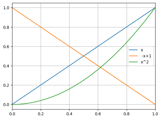
python -m chplot x " -x+1""x^2"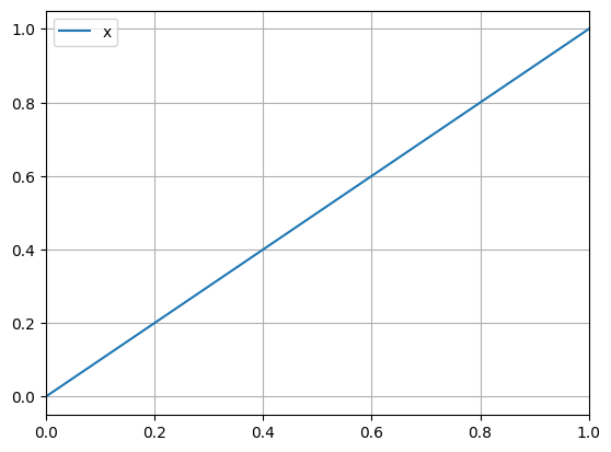

python -m chplot resources/files/equations.txt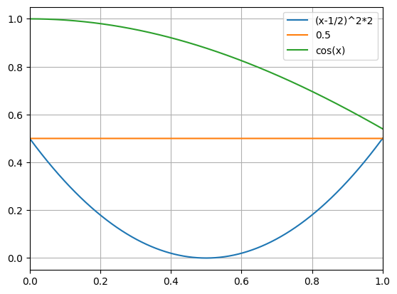

---

-v parameter

python -m chplot t(t-1) -v t
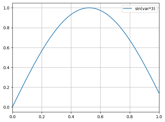
python -m chplot sin(var*3) -v var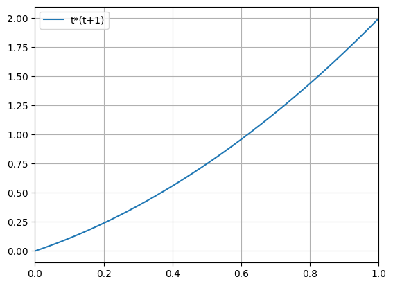

---

Overriding constant with variable:

python -m chplot c
python -m chplot c -v c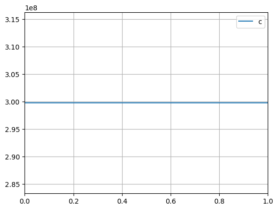

---

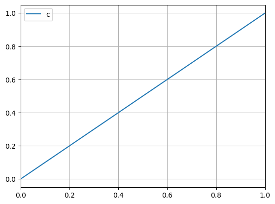
--no-sn

The expression in the first command is interpreted as $x\times1.2\cdot10^{-1}=0.12x$, and as $1.2\mathrm{e}\cdot x - 1$ in the second.

python -m chplot "x*1.2e-1"
python -m chplot "x*1.2e-1" --no-sn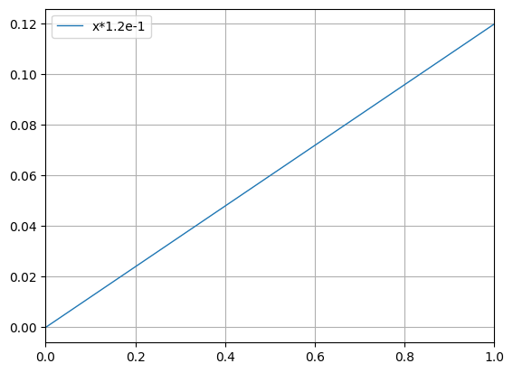

---

-x, -y parameters

Using expressions in the horizontal axis bounds:

python -m chplot "x^2+x" -x -3 3
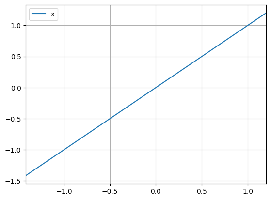
python -m chplot x -x " -sqrt(2)""zeta(3)"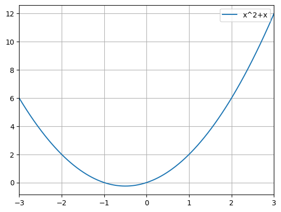

Using expressions in the vertical axis bounds and restricting the graph:

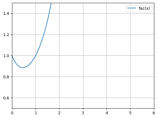
python -m chplot fac(x) -x 0 6
python -m chplot fac(x) -x 0 6 -y 0.5 1.5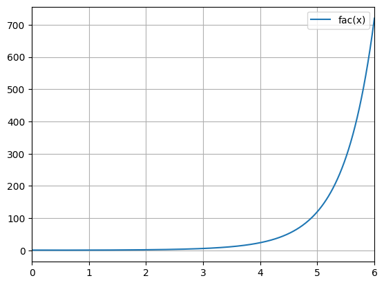

---

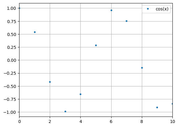
-n, -i, --dis parameters

The -i parameter removes the line between points.

python -m chplot cos(x) -x 0 10 -n 20
python -m chplot cos(x) -x 0 10 -i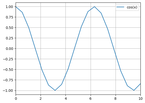

---

python -m chplot sqrt(x) -x 0 100 -i
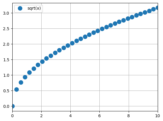
python -m chplot sqrt(x) -x 0 10 --dis 10 -n 35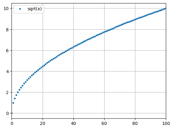

---

-xlog, -ylog parameters

python -m chplot "2^x" -x 1 100 -ylog
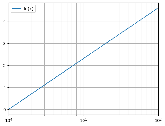
python -m chplot "ln(x)" -x 1 100 -xlog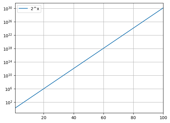

---

Log axis will adjust the bounds to remove negative points:

python -m chplot "x^3.5" -x 1 100 -xlog -ylog
python -m chplot "x" -x -5 5 -xlog
python -m chplot "x" -x -5 -1 -xlog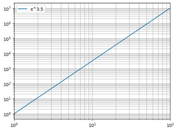

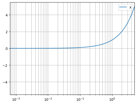
The second command generates a warning:

[CHPLOT] WARNING: x-axis scale is logarithmic, but its lower bound (-5.0) is negative, x-axis will be truncated to positive values

The third command generates en error:

[CHPLOT] CRITICAL: x-axis scale is logarithmic, but both its lower (-5.0) and upper (-1.0) bounds are negative, cannot graph anything

---

-z parameter

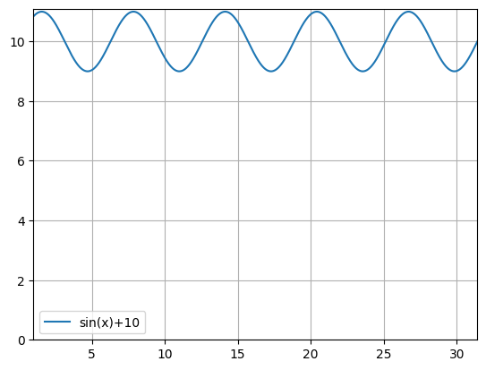
python -m chplot "sin(x)+10" -x 1 10pi
python -m chplot "sin(x)+10" -x 1 10pi -z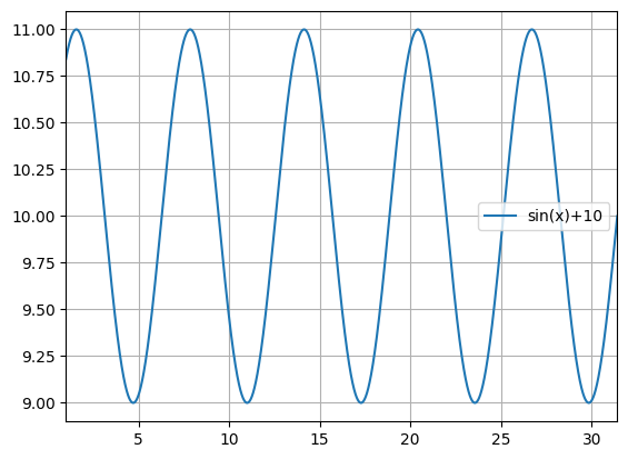

---

-xl, -yl, -t, -rl parameters

python -m chplot zeta(x) -x 1 10 -y 0 3
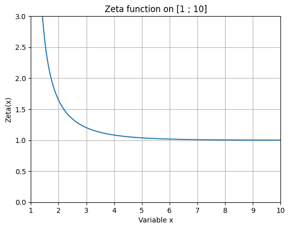
python -m chplot zeta(x) -x 1 10 -y 0 3 -xl "Variable x" -yl "Zeta(x)" -t "Zeta function on [1 ; 10]" -rl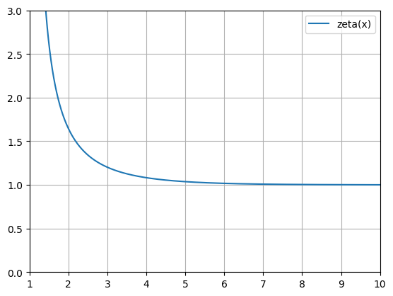

---

-square, -lw parameters

python -m chplot cbrt(x) --square
python -m chplot cbrt(x) -lw 5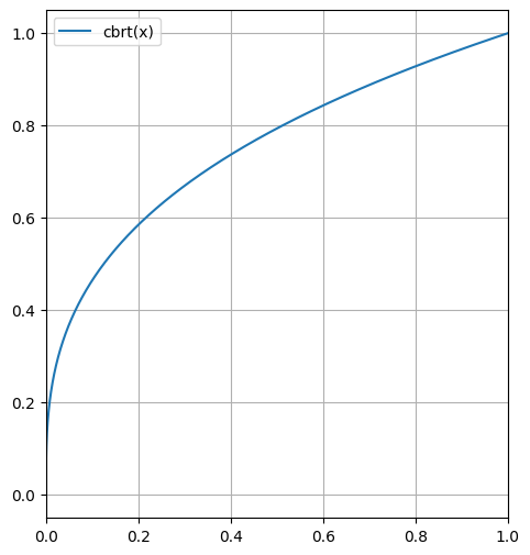

---

-c parameter

If a constant requires another one, define it after:

python -m chplot a*x+b -c a=2 b=7
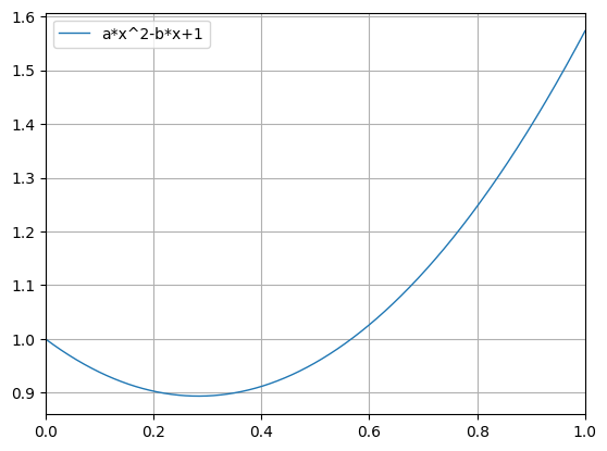
python -m chplot "a*x^2-b*x+1" -c a=8pi/19 "b=a^2-1"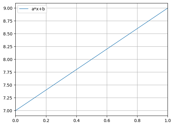

---

Constants can also be an expression, or come from a file:

python -m chplot cos(a*x) -c "a=(sqrt(2) - zeta(3)) / sin(1.5)" -x 0 50
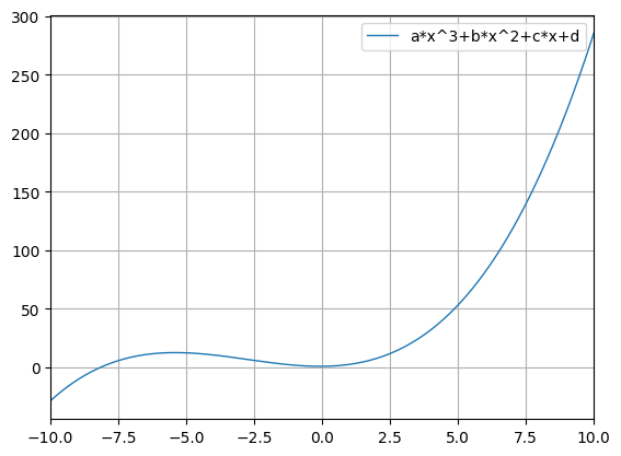
python -m chplot "a*x^3+b*x^2+c*x+d" -c resources\files\constants.txt -x -10 10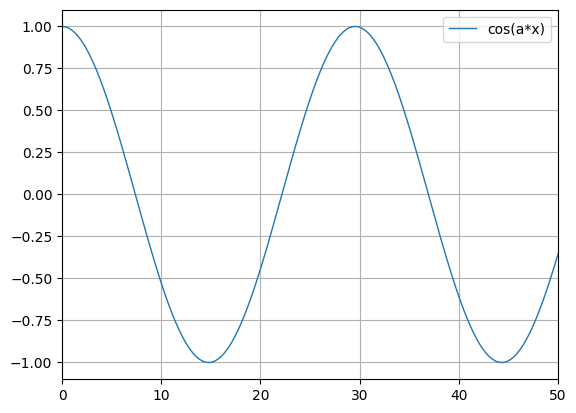

---

-f parameter

All the CSV format are summarized in the CSV files format section.

python -m chplot -f resources\files\data.csv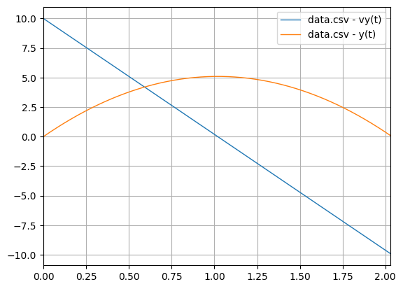

---

-d parameter

python -m chplot x "x(x+1)""x(x+1)(x+2)/2""x(x+1)(x+2)(x+3)/6" -d resources\files\saved_data.csv

The data can be found in the saved_data.csv file.

---

-p parameter

The file functions.py must be in the directory from where the command is executed.

python -m chplot "frac(x)+3""is_prime(x)""rnd(x, x/2)" -p functions.py -x 0 10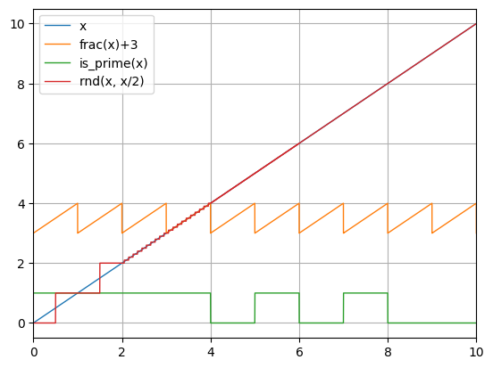

---

--zeros

python -m chplot sin(x) -x -7 7 --zeros
python -m chplot "x^2-2""in(x, 0.2, 0.3, 0, -2x+1)" -x 0 2 --zeros

The result of these commands (besides the plot) are the following. The first are the zeros of the function $\sin(x)$ on [-7 ; 7]: $\pm 2\pi$, $\pm \pi$ and $0$. Then the zero of $x^2-2$ is $\sqrt{2}$. Finally the last expression is completely zero on the interval [0.2 ; 0.3] and at $1/2$.

===== ZEROS OF THE FUNCTIONS =====
Note that non-continuous functions may give false zeros. Furthermore, some zeros may be missing if the graph is tangent to the x-axis.
- On the interval [-7.0 ; 7.0], the functionf(x) = sin(x) equals zero...
at x = -6.2831853072
at x = -3.1415926536
at x = 0.0
at x = 3.1415926536
at x = 6.2831853072

===== ZEROS OF THE FUNCTIONS =====
Note that non-continuous functions may give false zeros. Furthermore, some zeros may be missing if the graph is tangent to the x-axis.
- On the interval [0.0 ; 2.0], the functionf(x) = x^2-2 equals zero...
at x = 1.4142135624
- On the interval [0.0 ; 2.0], the functionf(x) = in(x, 0.2, 0.3, 0, -2x+1) equals zero...
on [0.2 ; 0.3]
at x = 0.5

---

--integral

python -m chplot "1/x" -x 1 e --integral
python -m chplot "x^2""exp(x)" --integral

The result of these commands (besides the plot) are the following.$$\int_1^e\frac{dx}{x} = 1$$ $$\int_0^1x^2dx = \frac{1}{3}$$$$\int_0^1\exp(x)dx=e - 1$$

===== INTEGRALS OF THE FUNCTIONS =====
Note that the more points, the smallest the error and that floating point numbers may introduce errors. Furthermore, discontinuous functions may indicate really huge error margins.
- ∫f(x)dx = 1.0000000021279944
where f(x) = 1/x on [1.0 ; 2.718]

===== INTEGRALS OF THE FUNCTIONS =====
Note that the more points, the smallest the error and that floating point numbers may introduce errors. Furthermore, discontinuous functions may indicate really huge error margins.
- ∫f(x)dx = 0.33333333499999834
where f(x) = x^2 on [0.0 ; 1.0]
- ∫f(x)dx = 1.7182818298909472
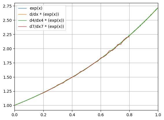
where f(x) = exp(x) on [0.0 ; 1.0]

---

--deriv parameter

The second command illustrates the instability of the higher order derivatives.

python -m chplot "sin(x)" --deriv 1 2 3 4 -x 0 4pi
python -m chplot "exp(x)" --deriv 1 4 7 -n 100000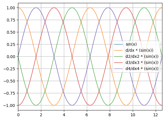

---

Synergy between --deriv and --zeros/--integral.

python -m chplot "x^2+2" -x -3 3 --deriv 1 --zeros --integral

===== ZEROS OF THE FUNCTIONS =====
Note that non-continuous functions may give false zeros. Furthermore, some zeros may be missing if the graph is tangent to the x-axis.
Furthermore, on derivatives and file data, zeros are approximated using linear interpolation, and may be far from their real values.
- On the interval [-3.0 ; 3.0], the functionf(x) = x^2+2 never equals zero.
- On the interval [-2.998 ; 2.998], the functionf(x) = d/dx * (x^2+2) equals zero...
at x = 0.0
===== INTEGRALS OF THE FUNCTIONS =====
Note that the more points, the smallest the error and that floating point numbers may introduce errors. Furthermore, discontinuous functions may indicate really huge error margins.
The x-axis limits on derivatives are slightly tighter because of the algorithm used. This may be counteracted by adding more points.
- ∫f(x)dx = 30.000000359996804
where f(x) = x^2+2 on [-3.0 ; 3.0]
- ∫f(x)dx = 6.18809004038144e-14
where f(x) = d/dx * (x^2+2) on [-2.998 ; 2.998]

---

--reg

Default keyword usable in the CLI.

python -m chplot "sin(x)"" -exp(x)" --reg lin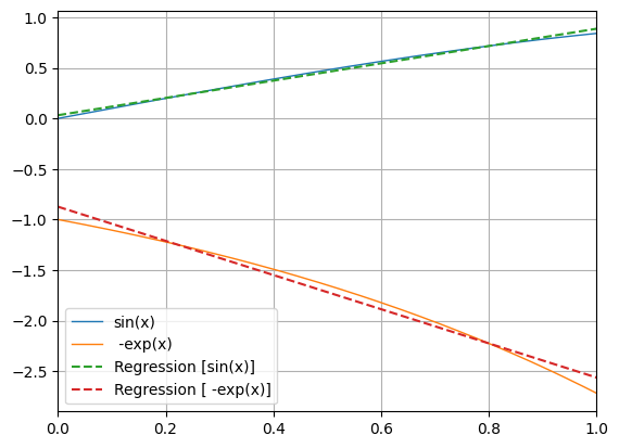

===== REGRESSION COEFFICIENTS OF THE FUNCTIONS =====
Regression function: reg(x) = a * x + b
- Function f(x) = sin(x)
Coefficients:
a = 0.85583 (exact 0.8558336726408089)
b = 0.03178 (exact 0.031776961574734974)
Accuracy on [0.000 ; 1.000]:
R2 = 0.9948573993162803
|err|<= 0.046139649407647365
|rel err|<= 317.625449951033
Copyable expression:
f(x) = (0.8558336726408089) * x + (0.031776961574734974)
- Function f(x) = -exp(x)
Coefficients:
a = -1.69032 (exact -1.6903174201716293)
b = -0.87314 (exact -0.8731372047610497)
Accuracy on [0.000 ; 1.000]:
R2 = 0.9837173025833181
|err|<= 0.15482720352636603
|rel err|<= 0.12686279523895028
Copyable expression:
f(x) = (-1.6903174201716293) * x + (-0.8731372047610497)

---

Arbitrary expression for regression (here: $a + \frac{b}{x} + \frac{c}{x^2}$).

python -m chplot "x""x^2-3x+2" -x 1 2 --reg "_ra + _rb/x + _rc/x^2"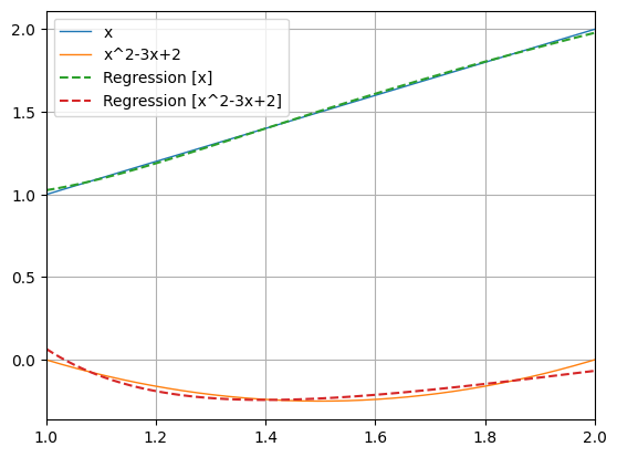

===== REGRESSION COEFFICIENTS OF THE FUNCTIONS =====
Regression function: reg(x) = a + b/x + c/x^2
- Function f(x) = x
Coefficients:
a = 4.32347 (exact 4.323472460240034)
b = -6.08251 (exact -6.082510526066791)
c = 2.7852 (exact 2.7852046542434103)
Accuracy on [1.000 ; 2.000]:
R2 = 0.9990492201082051
|err|<= 0.026166588416653536
|rel err|<= 0.026166588416653536
Copyable expression:
f(x) = (4.323472460240034) + (-6.082510526066791)/x + (2.7852046542434103)/x^2
- Function f(x) = x^2-3x+2
Coefficients:
a = 1.70398 (exact 1.7039810825081398)
b = -5.44646 (exact -5.446461246934391)
c = 3.8091 (exact 3.809103050454299)
Accuracy on [1.000 ; 2.000]:
R2 = 0.8852455638434826
|err|<= 0.06697377834548113
|rel err|<= 669.2141410779176
Copyable expression:
f(x) = (1.7039810825081398) + (-5.446461246934391)/x + (3.809103050454299)/x^2

---

Regression on file data.

python -m chplot -f resources\files\data.csv --reg poly2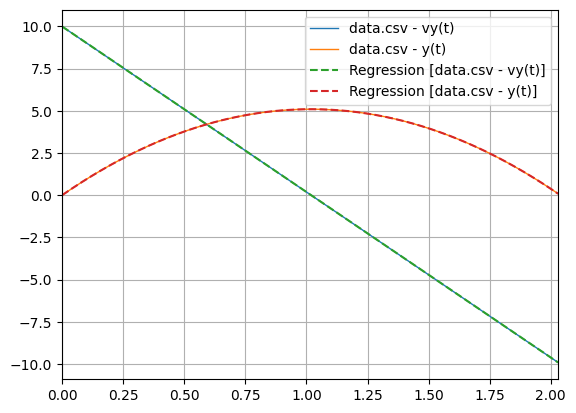

===== REGRESSION COEFFICIENTS OF THE FUNCTIONS =====
Regression function: reg(x) = a2 * x^2 + a1 * x + a0
- Function f(x) = data.csv - vy(t)
Coefficients:
a2 = 0.0 (exact -5.0979039530237654e-08)
a1 = -9.81 (exact -9.809999897491432)
a0 = 10.0 (exact 9.999999965897445)
Accuracy on [0.000 ; 2.030]:
R2 = 1.0
|err|<= 3.608967524826312e-08
|rel err|<= 2.809290005481242e-06
Copyable expression:
f(x) = (-5.0979039530237654e-08) * x^2 + (-9.809999897491432) * x + (9.999999965897445)
- Function f(x) = data.csv - y(t)
Coefficients:
a2 = -4.905 (exact -4.904999983961847)
a1 = 10.0 (exact 9.999999961872113)
a0 = 0.0 (exact 1.7338066957762713e-08)
Accuracy on [0.000 ; 2.030]:
R2 = 1.0
|err|<= 1.7338066957762713e-08
|rel err|<= 1.7041982824835924e-07
Copyable expression:
f(x) = (-4.904999983961847) * x^2 + (9.999999961872113) * x + (1.7338066957762713e-08)

---

Synergy between --reg and --deriv/--zeros/--integral.

python -m chplot log2(x) -x 1 3 --deriv 1 --reg lin --zeros --integral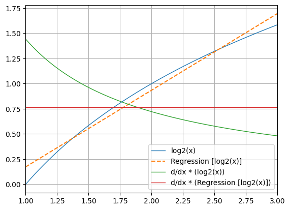

===== REGRESSION COEFFICIENTS OF THE FUNCTIONS =====
Regression function: reg(x) = a * x + b
- Function f(x) = log2(x)
Coefficients:
a = 0.76193 (exact 0.7619286641417374)
b = -0.58912 (exact -0.5891228449973627)
Accuracy on [1.000 ; 3.000]:
R2 = 0.9808243468285833
|err|<= 0.17280581914437476
|rel err|<= 598.4874010749205
Copyable expression:
f(x) = (0.7619286641417374) * x + (-0.5891228449973627)
===== ZEROS OF THE FUNCTIONS =====
Note that non-continuous functions may give false zeros. Furthermore, some zeros may be missing if the graph is tangent to the x-axis.
Furthermore, on derivatives and file data, zeros are approximated using linear interpolation, and may be far from their real values.
- On the interval [1.0 ; 3.0], the functionf(x) = log2(x) equals zero...
at x = 1.0
- On the interval [1.0 ; 3.0], the functionf(x) = Regression [log2(x)] never equals zero.
- On the interval [1.001 ; 2.999], the functionf(x) = d/dx * (log2(x)) never equals zero.
- On the interval [1.001 ; 2.999], the functionf(x) = d/dx * (Regression [log2(x)]) never equals zero.
===== INTEGRALS OF THE FUNCTIONS =====
Note that the more points, the smallest the error and that floating point numbers may introduce errors. Furthermore, discontinuous functions may indicate really huge error margins.
The x-axis limits on derivatives are slightly tighter because of the algorithm used. This may be counteracted by adding more points.
- ∫f(x)dx = 1.8694974171793488
where f(x) = log2(x) on [1.0 ; 3.0]
- ∫f(x)dx = 1.8694689665720188
where f(x) = Regression [log2(x)] on [1.0 ; 3.0]
- ∫f(x)dx = 1.583424040388957
where f(x) = d/dx * (log2(x)) on [1.001 ; 2.999]
- ∫f(x)dx = 1.5226382424208345
where f(x) = d/dx * (Regression [log2(x)]) on [1.001 ; 2.999]

Possible improvements

• Parallelizing computation of expressions.