The Python Toolbox for Neurophysiological Signal Processing

NeuroKit2 is a user-friendly package providing easy access to advanced biosignal processing routines. Researchers and clinicians without extensive knowledge of programming or biomedical signal processing can analyze physiological data with only two lines of code.

Quick Example

importneurokit2asnk# Download example datadata=nk.data("bio_eventrelated_100hz")
# Preprocess the data (filter, find peaks, etc.)processed_data, info=nk.bio_process(ecg=data["ECG"], rsp=data["RSP"], eda=data["EDA"], sampling_rate=100)
# Compute relevant featuresresults=nk.bio_analyze(processed_data, sampling_rate=100)

And boom 💥 your analysis is done 😎

Download

You can download NeuroKit2 from PyPI

pip install neurokit2

or conda-forge

conda install -c conda-forge neurokit2

If you're not sure what to do, read our installation guide.

Contributing

NeuroKit2 is the most welcoming project with a large community of contributors with all levels of programming expertise. But the package is still far from being perfect! Thus, if you have some ideas for improvement, new features, or just want to learn Python and do something useful at the same time, do not hesitate and check out the following guide:

• Contributing to NeuroKit

Also, if you have developed new signal processing methods or algorithms and you want to increase their usage, popularity, and citations, get in touch with us to eventually add them to NeuroKit. A great opportunity for the users as well as the original developers!

You have spotted a mistake? An error in a formula or code? OR there is just a step that seems strange and you don't understand? Please let us know! We are human beings, and we'll appreciate any inquiry.

Documentation

Click on the links above and check out our tutorials:

General

• Get familiar with Python in 10 minutes
• Recording good quality signals
• Install Python and NeuroKit
• Included datasets
• Additional Resources

Examples

• Simulate Artificial Physiological Signals
• Customize your Processing Pipeline
• Event-related Analysis
• Interval-related Analysis
• Analyze Electrodermal Activity (EDA)
• Analyze Respiratory Rate Variability (RRV)
• Extract and Visualize Individual Heartbeats
• Locate P, Q, S, and T waves in ECG
• Analyze Electrooculography EOG data

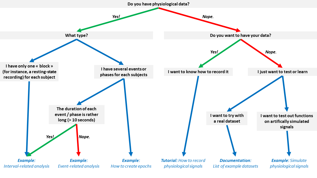
Don't know which tutorial is suited for your case? Follow this flowchart:

Citation

The NeuroKit2 paper can be found here 🎉 Additionally, you can get the reference directly from Python by running:

nk.cite()

You can cite NeuroKit2 as follows:
- Makowski, D., Pham, T., Lau, Z. J., Brammer, J. C., Lespinasse, F., Pham, H.,
Schölzel, C., & Chen, S. A. (2021). NeuroKit2: A Python toolbox for neurophysiological signal processing.
Behavior Research Methods, 53(4), 1689–1696. https://doi.org/10.3758/s13428-020-01516-y
Full bibtex reference:
@article{Makowski2021neurokit,
author = {Dominique Makowski and Tam Pham and Zen J. Lau and Jan C. Brammer and Fran{\c{c}}ois Lespinasse and Hung Pham and Christopher Schölzel and S. H. Annabel Chen},
title = {{NeuroKit}2: A Python toolbox for neurophysiological signal processing},
journal = {Behavior Research Methods},
volume = {53},
number = {4},
pages = {1689--1696},
publisher = {Springer Science and Business Media {LLC}},
doi = {10.3758/s13428-020-01516-y},
url = {https://doi.org/10.3758%2Fs13428-020-01516-y},
year = 2021,
month = {feb}
}

Let us know if you used NeuroKit2 in a publication! Open a new discussion (select the NK in publications category) and link the paper. The community would be happy to know about how you used it and learn about your research. We could also feature it once we have a section on the website for papers that used the software.

Physiological Data Preprocessing

Simulate physiological signals

You can easily simulate artificial ECG (also 12-Lead multichannel ECGs), PPG, RSP, EDA, and EMG signals to test your scripts and algorithms.

importnumpyasnpimportpandasaspdimportneurokit2asnk# Generate synthetic signalsecg=nk.ecg_simulate(duration=10, heart_rate=70)
ppg=nk.ppg_simulate(duration=10, heart_rate=70)
rsp=nk.rsp_simulate(duration=10, respiratory_rate=15)
eda=nk.eda_simulate(duration=10, scr_number=3)
emg=nk.emg_simulate(duration=10, burst_number=2)
# Visualise biosignalsdata=pd.DataFrame({"ECG": ecg,
"PPG": ppg,
"RSP": rsp,
"EDA": eda,
"EMG": emg})
nk.signal_plot(data, subplots=True)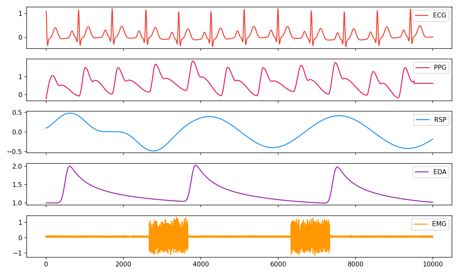

Electrodermal Activity (EDA/GSR)

# Generate 10 seconds of EDA signal (recorded at 250 samples / second) with 2 SCR peakseda=nk.eda_simulate(duration=10, sampling_rate=250, scr_number=2, drift=0.01)
# Process itsignals, info=nk.eda_process(eda, sampling_rate=250)
# Visualise the processingnk.eda_plot(signals, info)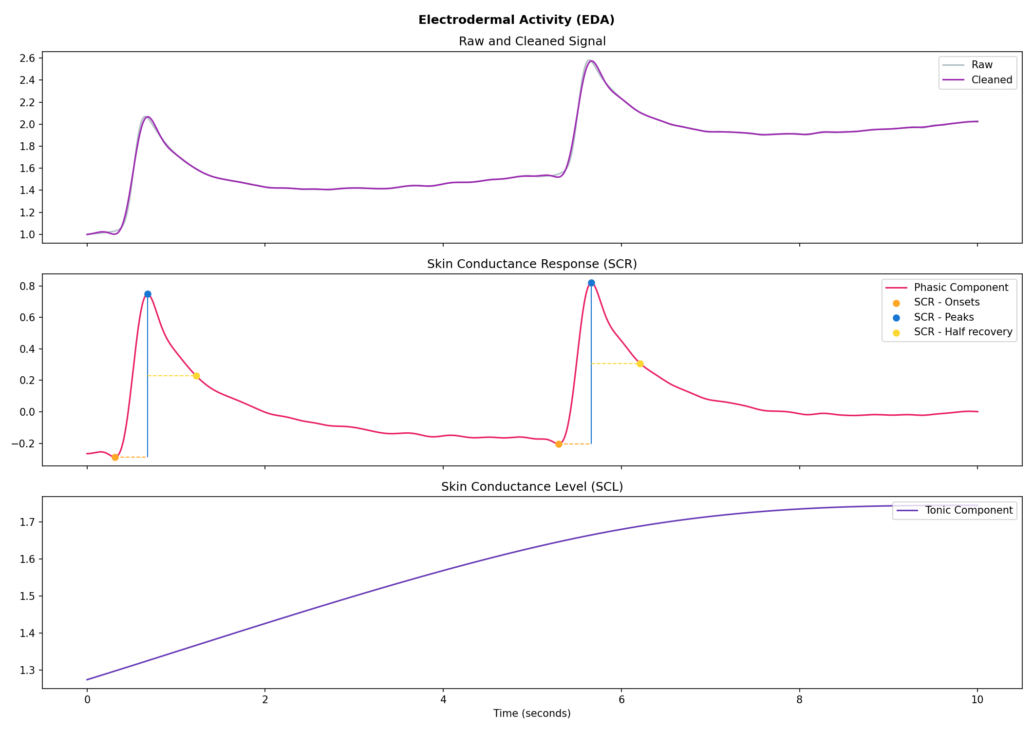

Cardiac activity (ECG)

# Generate 15 seconds of ECG signal (recorded at 250 samples/second)ecg=nk.ecg_simulate(duration=15, sampling_rate=250, heart_rate=70)
# Process itsignals, info=nk.ecg_process(ecg, sampling_rate=250)
# Visualise the processingnk.ecg_plot(signals, info)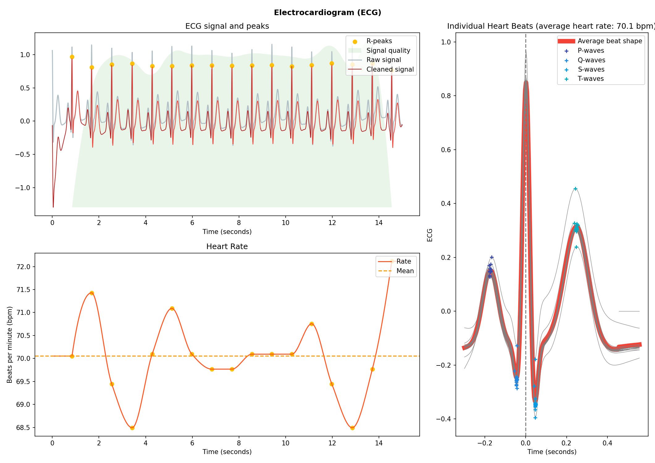

Respiration (RSP)

# Generate one minute of respiratory (RSP) signal (recorded at 250 samples / second)rsp=nk.rsp_simulate(duration=60, sampling_rate=250, respiratory_rate=15)
# Process itsignals, info=nk.rsp_process(rsp, sampling_rate=250)
# Visualise the processingnk.rsp_plot(signals, info)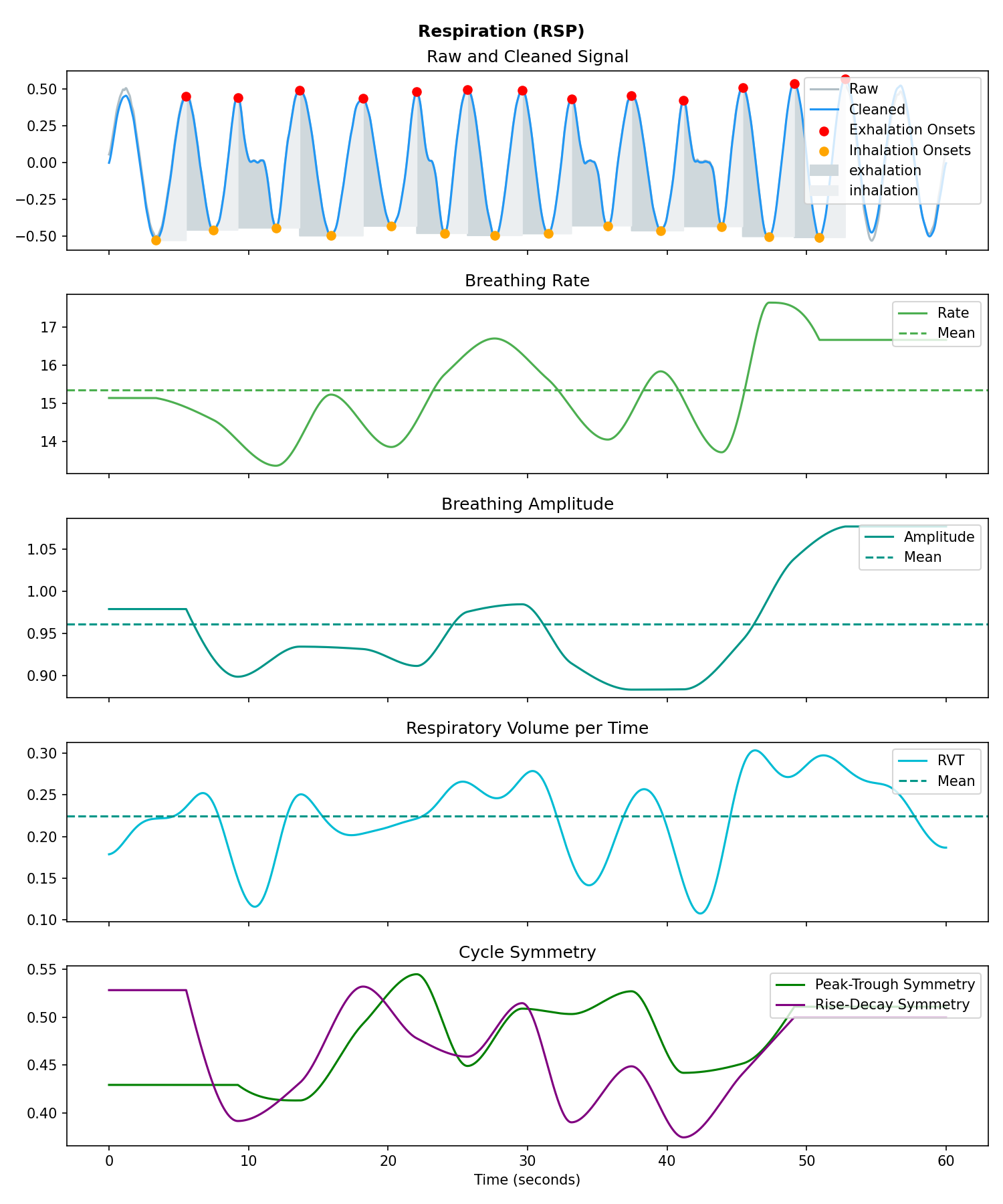

Photoplethysmography (PPG/BVP)

# Generate 15 seconds of PPG signal (recorded at 250 samples/second)ppg=nk.ppg_simulate(duration=15, sampling_rate=250, heart_rate=70)
# Process itsignals, info=nk.ppg_process(ppg, sampling_rate=250)
# Visualize the processingnk.ppg_plot(signals, info)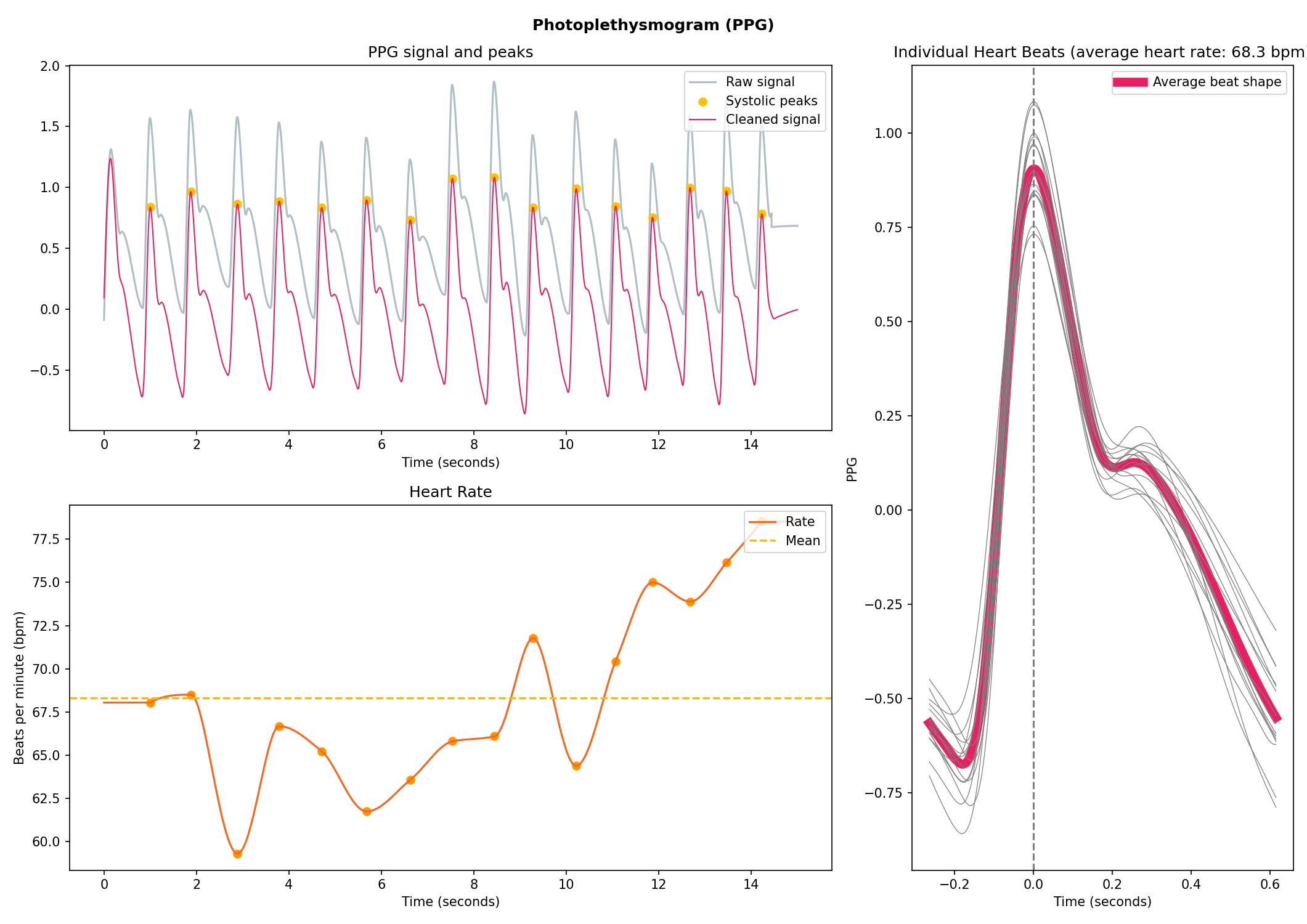

Electromyography (EMG)

# Generate 10 seconds of EMG signal (recorded at 250 samples/second)emg=nk.emg_simulate(duration=10, sampling_rate=250, burst_number=3)
# Process itsignals, info=nk.emg_process(emg, sampling_rate=250)
# Visualise the processingnk.emg_plot(signals, info)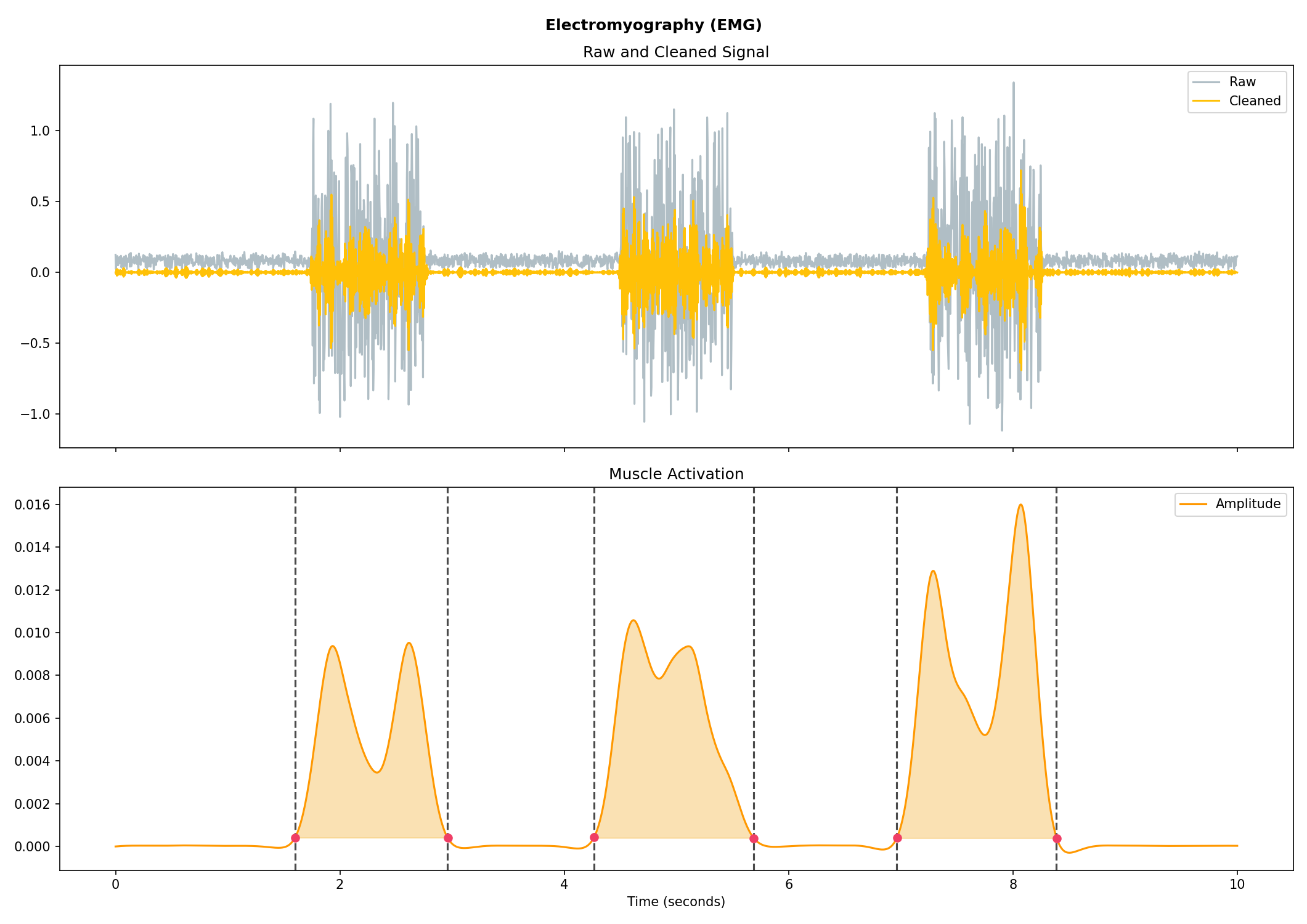

Electrooculography (EOG)

# Import EOG dataeog_signal=nk.data("eog_100hz")
# Process itsignals, info=nk.eog_process(eog_signal, sampling_rate=100)
# Plotnk.eog_plot(signals, info)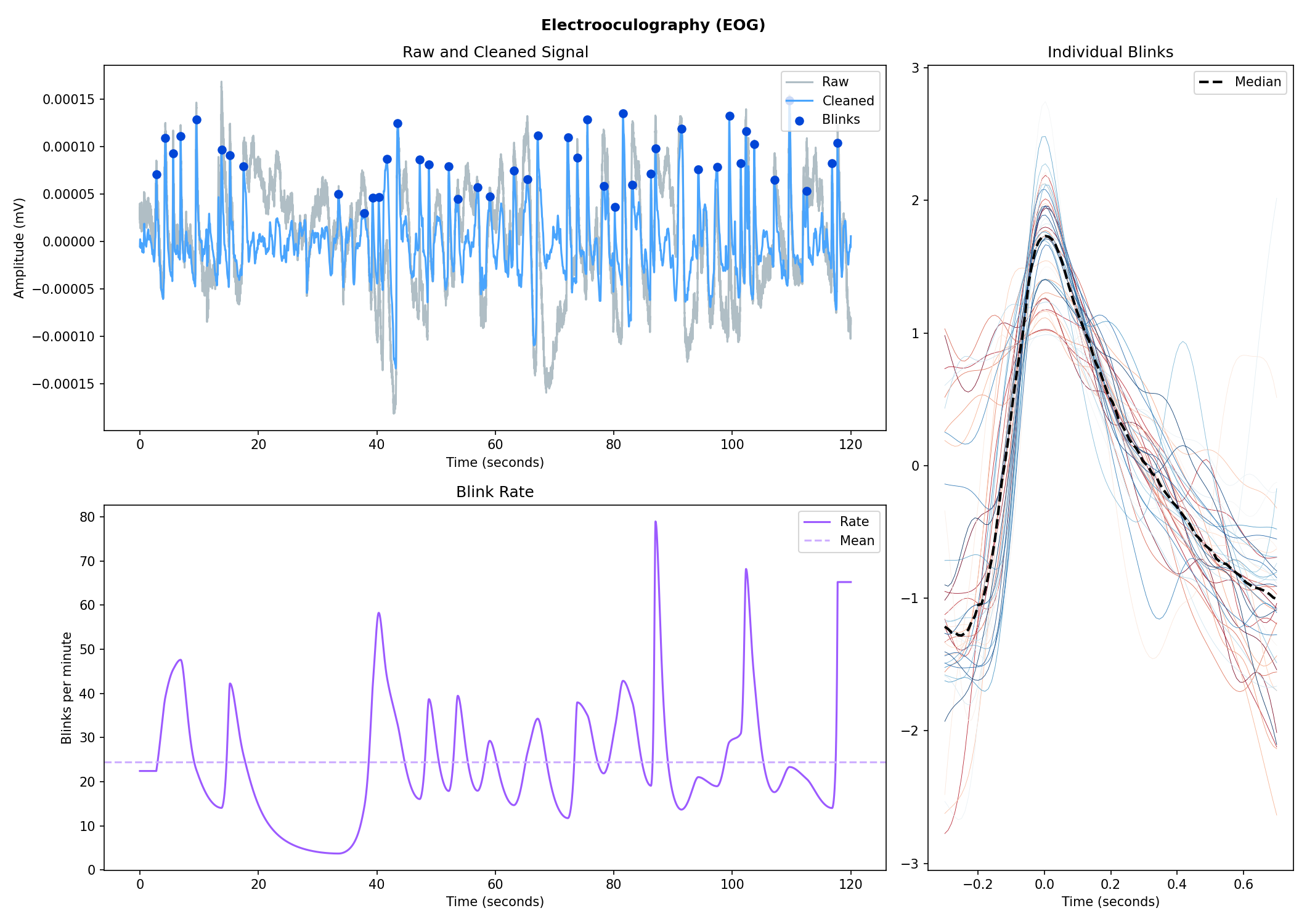

Electrogastrography (EGG)

Consider helping us develop it!

Physiological Data Analysis

The analysis of physiological data usually comes in two types, event-related or interval-related.

Event-related

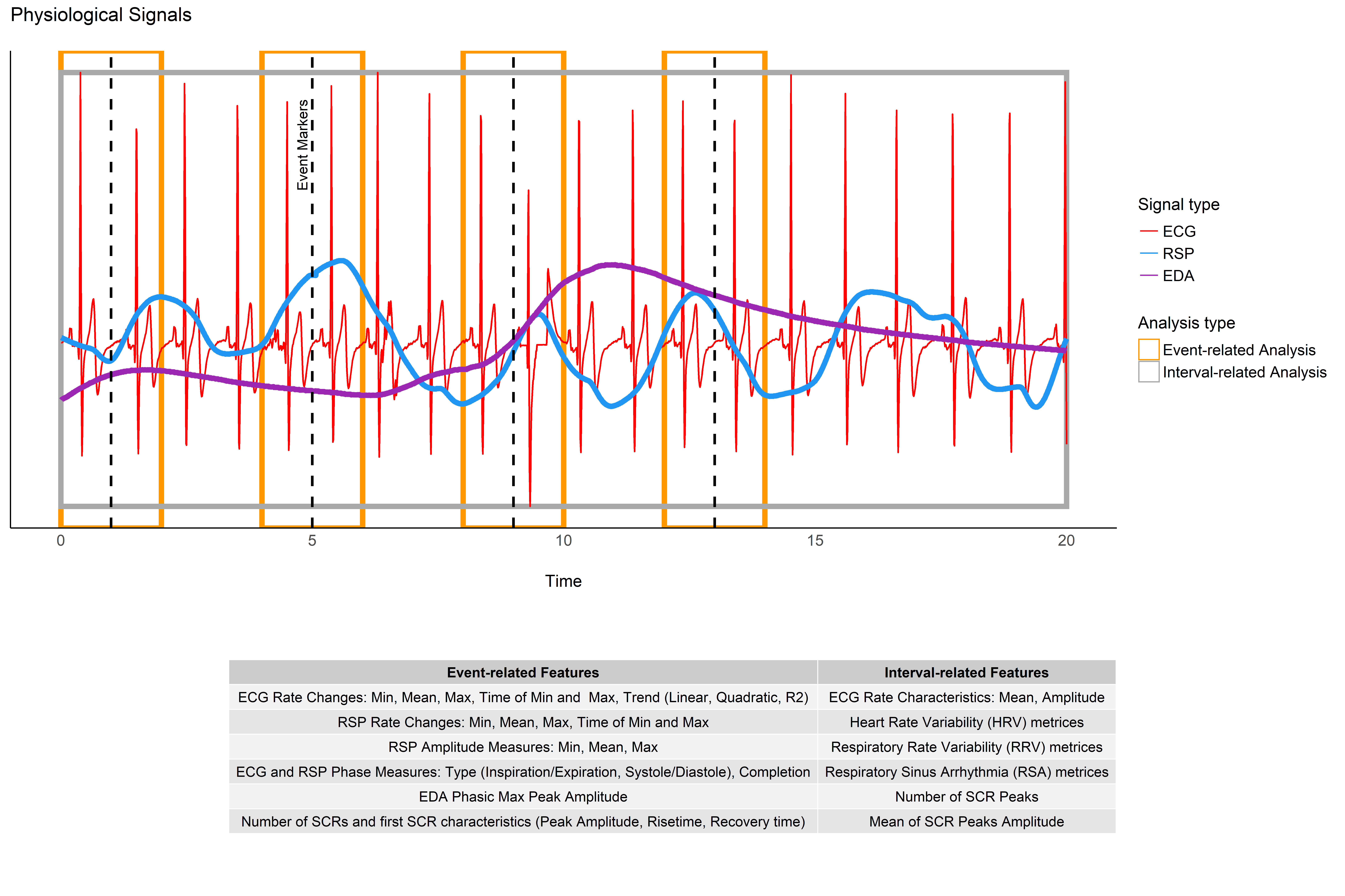
This type of analysis refers to physiological changes immediately occurring in response to an event. For instance, physiological changes following the presentation of a stimulus (e.g., an emotional stimulus) are indicated by the dotted lines in the figure above. In this situation, the analysis is epoch-based. An epoch is a short chunk of the physiological signal (usually < 10 seconds), that is locked to a specific stimulus and hence the physiological signals of interest are time-segmented accordingly. This is represented by the orange boxes in the figure above. In this case, using bio_analyze() will compute features like rate changes, peak characteristics, and phase characteristics.

• Event-related example

Interval-related

This type of analysis refers to the physiological characteristics and features that occur over longer periods of time (from a few seconds to days of activity). Typical use cases are either periods of resting state, in which the activity is recorded for several minutes while the participant is at rest, or during different conditions in which there is no specific time-locked event (e.g., watching movies, listening to music, engaging in physical activity, etc.). For instance, this type of analysis is used when people want to compare the physiological activity under different intensities of physical exercise, different types of movies, or different intensities of stress. To compare event-related and interval-related analysis, we can refer to the example figure above. For example, a participant might be watching a 20s-long short film where particular stimuli of interest in the movie appear at certain time points (marked by the dotted lines). While event-related analysis pertains to the segments of signals within the orange boxes (to understand the physiological changes pertaining to the appearance of stimuli), interval-related analysis can be applied on the entire 20s duration to investigate how physiology fluctuates in general. In this case, using bio_analyze() will compute features such as rate characteristics (in particular, variability metrics) and peak characteristics.

• Interval-related example

Heart Rate Variability (HRV)

Check-out our Heart Rate Variability in Psychology: A Review of HRV Indices and an Analysis Tutorialpaper for:

• a comprehensive review of the most up-to-date HRV indices
• a discussion of their significance in psychological research and practices
• a step-by-step guide for HRV analysis using NeuroKit2

You can cite the paper as follows:
- Pham, T., Lau, Z. J., Chen, S. H. A., & Makowski, D. (2021).
Heart Rate Variability in Psychology: A Review of HRV Indices and an Analysis Tutorial.
Sensors, 21(12), 3998. https://doi:10.3390/s21123998

• Compute HRV indices using Python
  • Time domain: RMSSD, MeanNN, SDNN, SDSD, CVNN, etc.
  • Frequency domain: Spectral power density in various frequency bands (Ultra low/ULF, Very low/VLF, Low/LF, High/HF, Very high/VHF), Ratio of LF to HF power, Normalized LF (LFn) and HF (HFn), Log transformed HF (LnHF).
  • Nonlinear domain: Spread of RR intervals (SD1, SD2, ratio between SD2 to SD1), Cardiac Sympathetic Index (CSI), Cardial Vagal Index (CVI), Modified CSI, Sample Entropy (SampEn).

# Download datadata=nk.data("bio_resting_8min_100hz")
# Find peakspeaks, info=nk.ecg_peaks(data["ECG"], sampling_rate=100)
# Compute HRV indicesnk.hrv(peaks, sampling_rate=100, show=True)
>>>HRV_RMSSDHRV_MeanNNHRV_SDNN ... HRV_CVIHRV_CSI_ModifiedHRV_SampEn>>>069.697983696.39534962.135891 ... 4.829101592.0953721.259931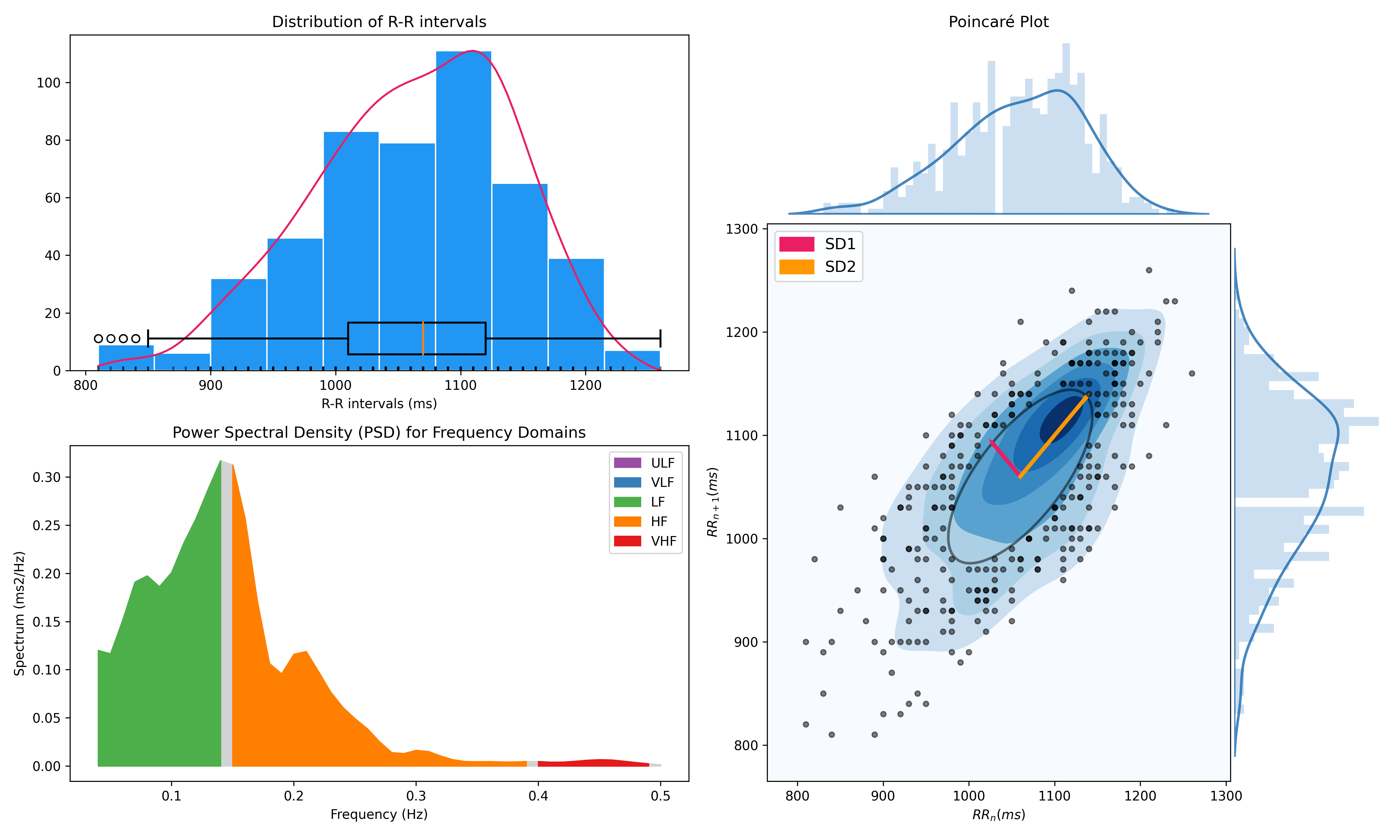

Miscellaneous

ECG Delineation

• Delineate the QRS complex of an electrocardiac signal (ECG) including P-peaks, T-peaks, as well as their onsets and offsets.

# Download dataecg_signal=nk.data(dataset="ecg_3000hz")
# Extract R-peaks locations_, rpeaks=nk.ecg_peaks(ecg_signal, sampling_rate=3000)
# Delineatesignal, waves=nk.ecg_delineate(ecg_signal, rpeaks, sampling_rate=3000, method="dwt", show=True, show_type='all')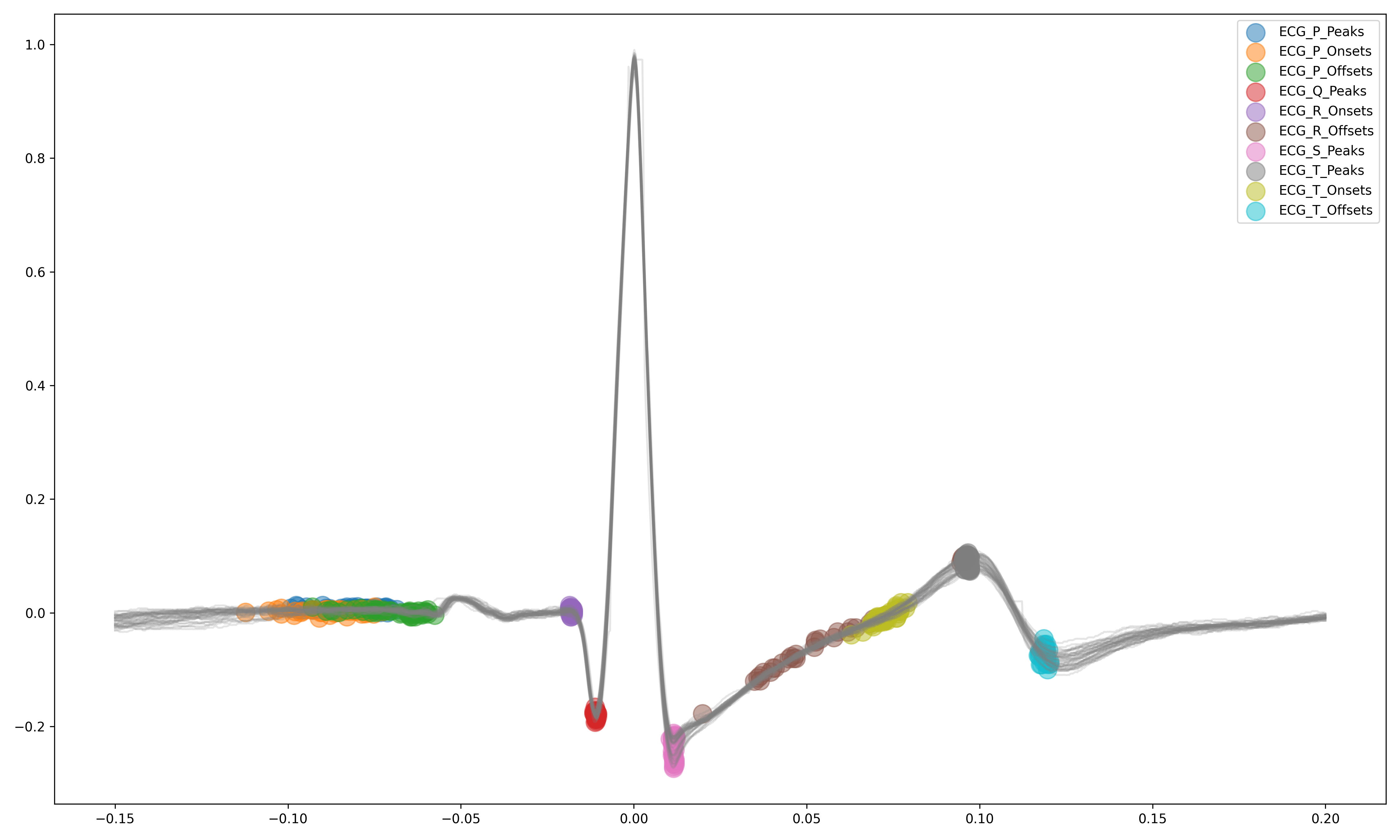

Signal Processing

• Signal processing functionalities
  • Filtering: Using different methods.
  • Detrending: Remove the baseline drift or trend.
  • Distorting: Add noise and artifacts.

# Generate original signaloriginal=nk.signal_simulate(duration=6, frequency=1)
# Distort the signal (add noise, linear trend, artifacts, etc.)distorted=nk.signal_distort(original,
noise_amplitude=0.1,
noise_frequency=[5, 10, 20],
powerline_amplitude=0.05,
artifacts_amplitude=0.3,
artifacts_number=3,
linear_drift=0.5)
# Clean (filter and detrend)cleaned=nk.signal_detrend(distorted)
cleaned=nk.signal_filter(cleaned, lowcut=0.5, highcut=1.5)
# Compare the 3 signalsplot=nk.signal_plot([original, distorted, cleaned])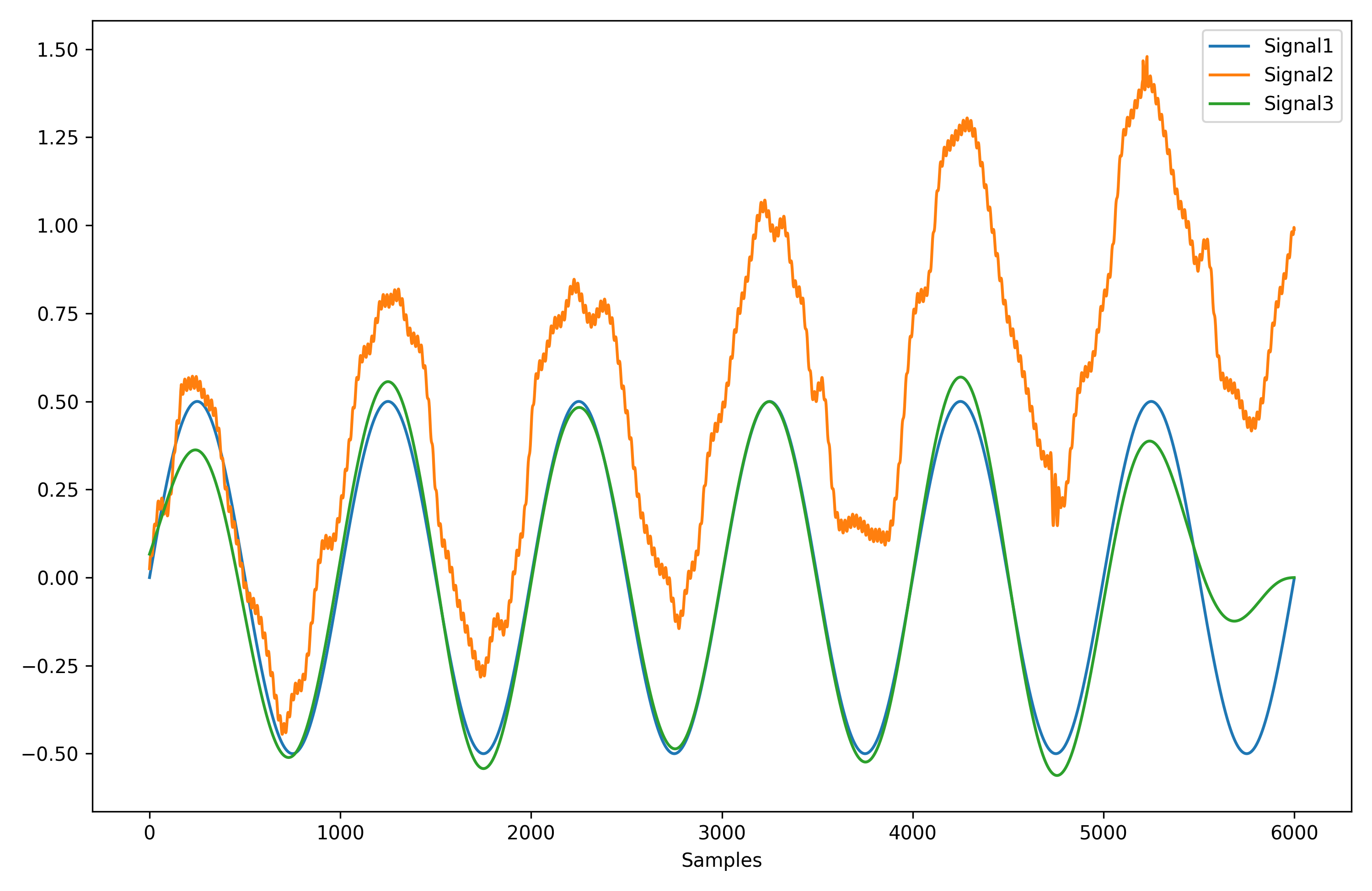

Complexity (Entropy, Fractal Dimensions, ...)

• Optimize complexity parameters (delay tau, dimension m, tolerance r)

# Generate signalsignal=nk.signal_simulate(frequency=[1, 3], noise=0.01, sampling_rate=200)
# Find optimal time delay, embedding dimension, and rparameters=nk.complexity_optimize(signal, show=True)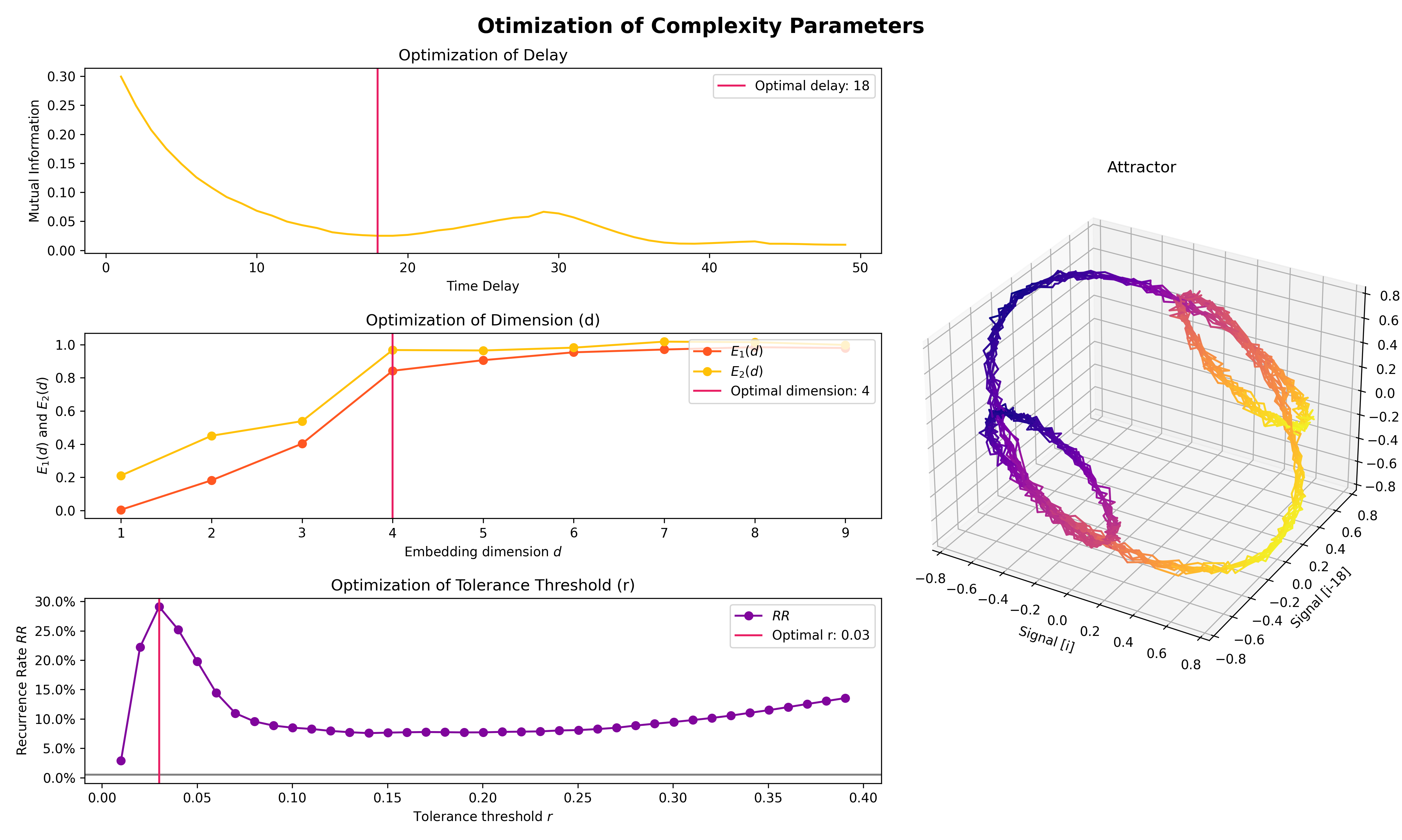

• Compute complexity features
  • Entropy: Sample Entropy (SampEn), Approximate Entropy (ApEn), Fuzzy Entropy (FuzzEn), Multiscale Entropy (MSE), Shannon Entropy (ShEn)
  • Fractal dimensions: Correlation Dimension D2, ...
  • Detrended Fluctuation Analysis

nk.entropy_sample(signal)
nk.entropy_approximate(signal)

Signal Decomposition

# Create complex signalsignal=nk.signal_simulate(duration=10, frequency=1) # High freqsignal+=3*nk.signal_simulate(duration=10, frequency=3) # Higher freqsignal+=3*np.linspace(0, 2, len(signal)) # Add baseline and linear trendsignal+=2*nk.signal_simulate(duration=10, frequency=0.1, noise=0) # Non-linear trendsignal+=np.random.normal(0, 0.02, len(signal)) # Add noise# Decompose signal using Empirical Mode Decomposition (EMD)components=nk.signal_decompose(signal, method='emd')
nk.signal_plot(components) # Visualize components# Recompose merging correlated componentsrecomposed=nk.signal_recompose(components, threshold=0.99)
nk.signal_plot(recomposed) # Visualize components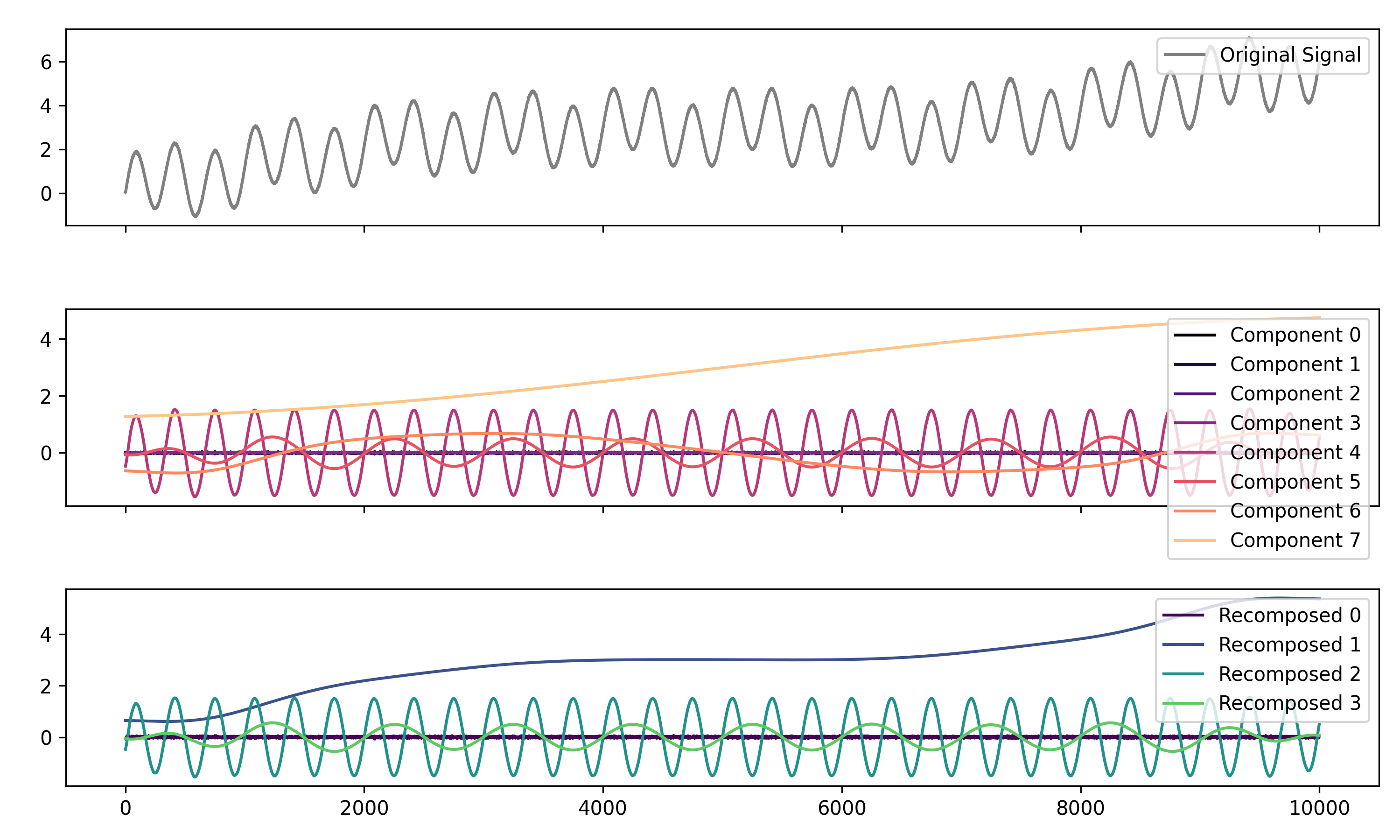

Signal Power Spectrum Density (PSD)

# Generate complex signalsignal=nk.signal_simulate(duration=20, frequency=[0.5, 5, 10, 15], amplitude=[2, 1.5, 0.5, 0.3], noise=0.025)
# Get the PSD using different methodswelch=nk.signal_psd(signal, method="welch", min_frequency=1, max_frequency=20, show=True)
multitaper=nk.signal_psd(signal, method="multitapers", max_frequency=20, show=True)
lomb=nk.signal_psd(signal, method="lomb", min_frequency=1, max_frequency=20, show=True)
burg=nk.signal_psd(signal, method="burg", min_frequency=1, max_frequency=20, order=10, show=True)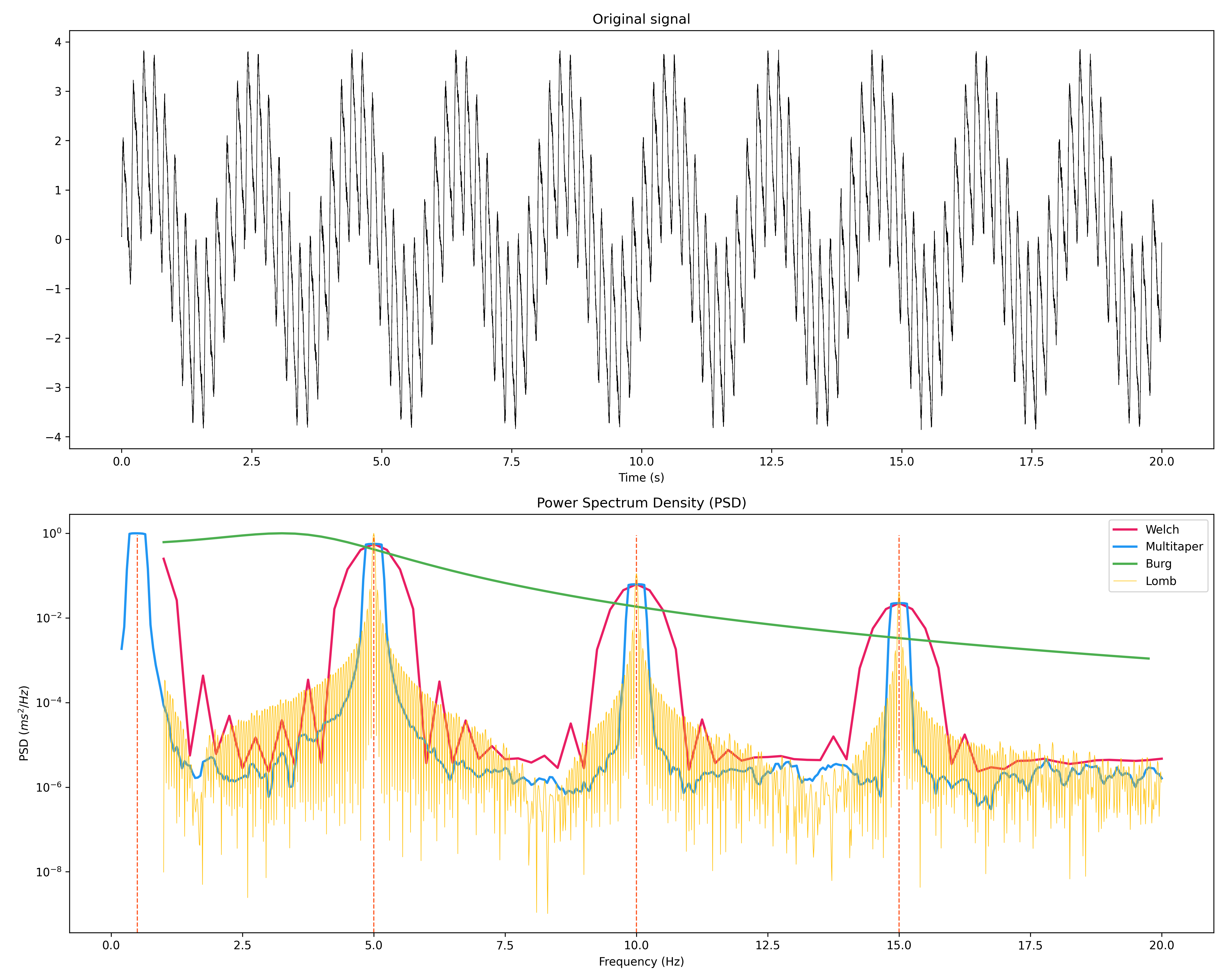

Statistics

• Highest Density Interval (HDI)

x=np.random.normal(loc=0, scale=1, size=100000)
ci_min, ci_max=nk.hdi(x, ci=0.95, show=True)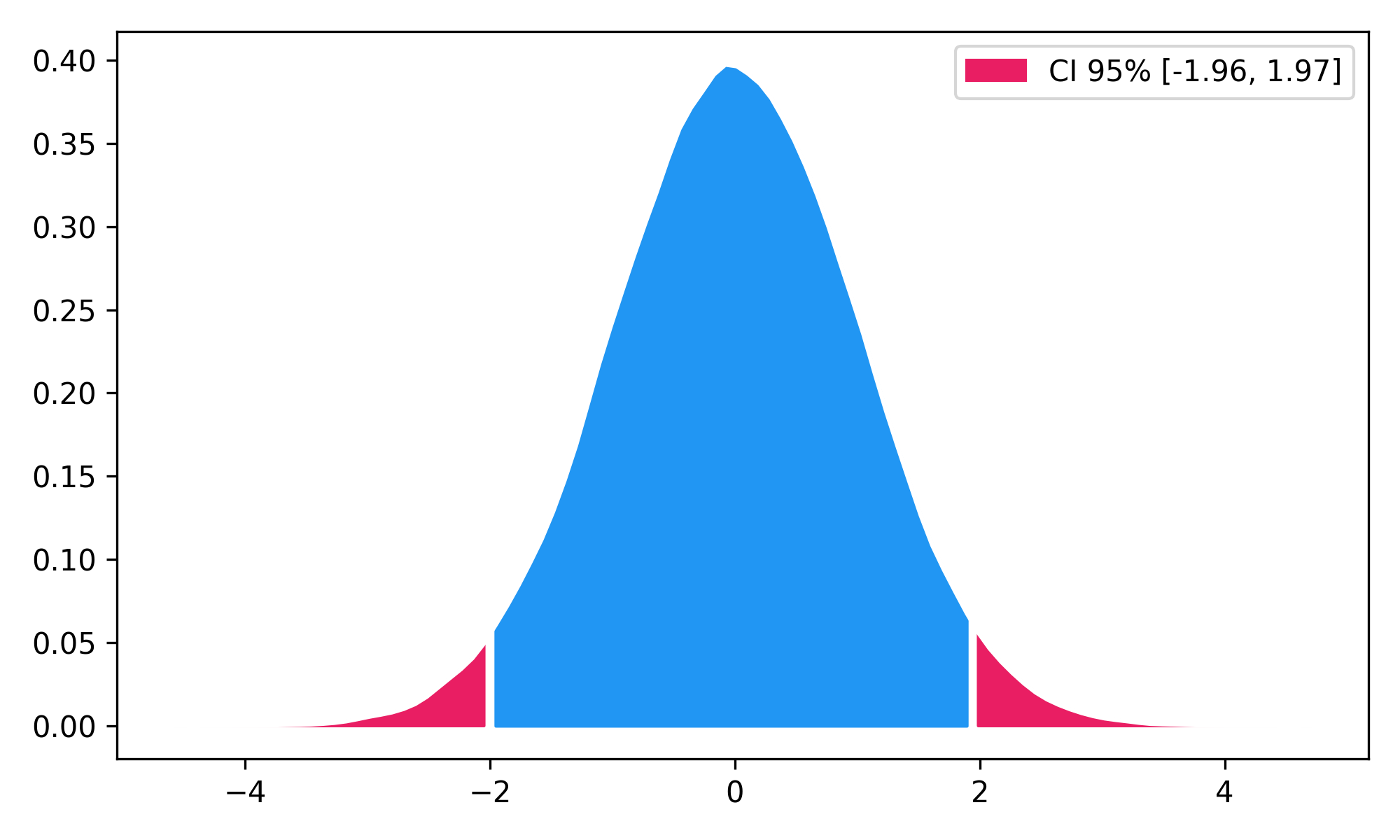

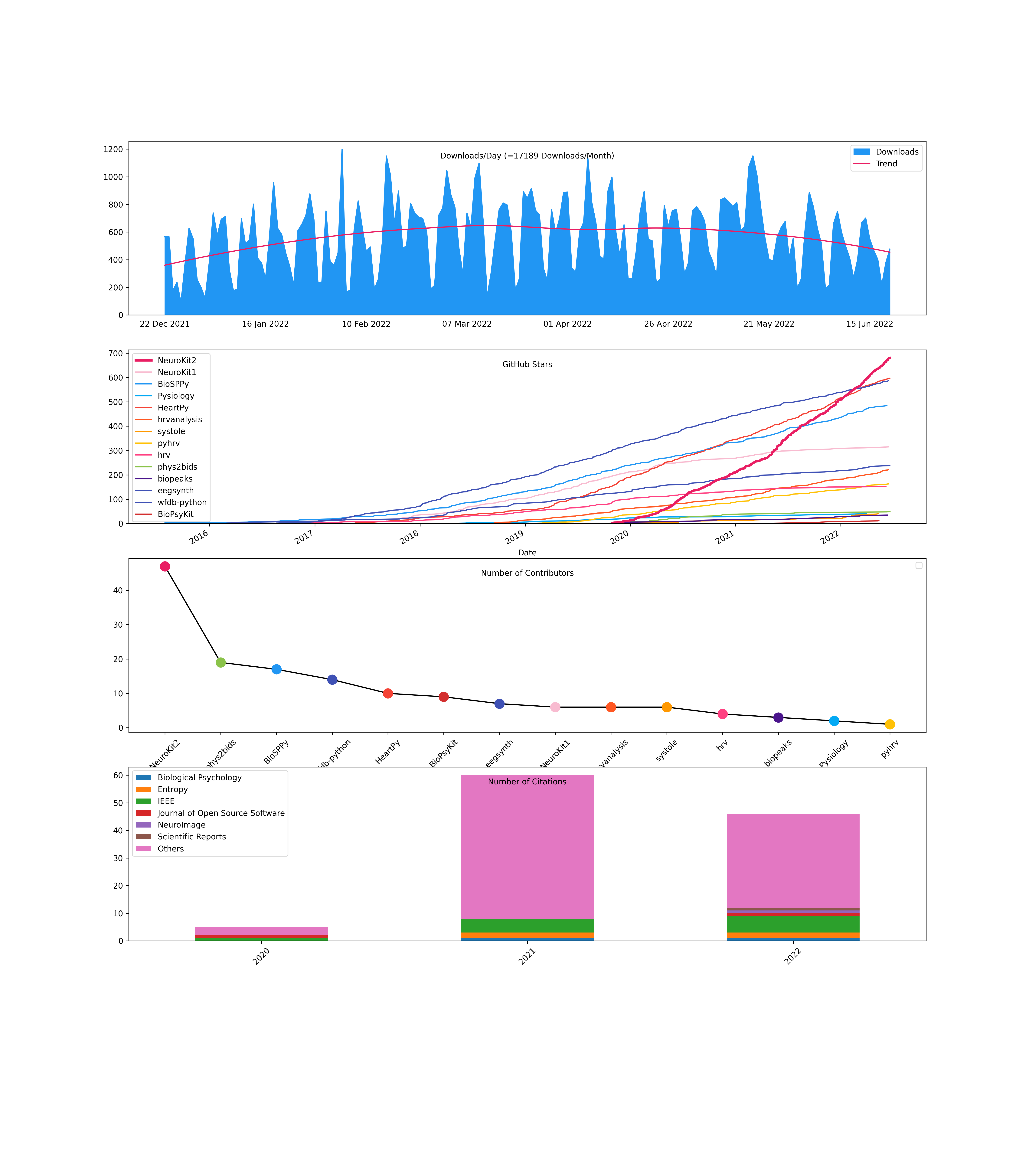
Popularity

NeuroKit2 is one of the most welcoming packages for new contributors and users, as well as the fastest-growing package. So stop hesitating and hop on board 🤗

Used at

Disclaimer

The authors do not provide any warranty. If this software causes your keyboard to blow up, your brain to liquefy, your toilet to clog or a zombie plague to break loose, the authors CANNOT IN ANY WAY be held responsible.