- TensorFlow
- RNN循环神经网络
- 官网:https://www.tensorflow.org/
- TensorFlow是Google开发的一款神经网络的Python外部的结构包, 也是一个采用数据流图来进行数值计算的开源软件库.
- 先绘制计算结构图, 也可以称是一系列可人机交互的计算操作, 然后把编辑好的Python文件 转换成 更高效的C++, 并在后端进行计算.
- 擅长的任务就是训练深度神经网络
- 快速的入门神经网络,大大降低了深度学习(也就是深度神经网络)的开发成本和开发难度
- TensorFlow 的开源性, 让所有人都能使用并且维护
- 暂不支持Windows下安装TensorFlow,可以在虚拟机里使用或者安装Docker安装
- 这里在CentOS6.5下进行安装
- 安装Python2.7,默认CentOS中安装的是Python2.6
- 先安装zlib的依赖,下面安装easy_install时会用到
yum install zlib
yum install zlib-devel
- 在安装openssl的依赖,下面安装pip时会用到
yum install openssl
yum install openssl-devel
- 下载安装包,我传到
github上的安装包,https协议后面加上--no-check-certificate,:
wget https://raw.githubusercontent.com/lawlite19/LinuxSoftware/master/python/Python-2.7.12.tgz --no-check-certificate
- 解压缩:
tar -zxvf xxx - 进入,配置:
./configure --prefix=/usr/local/python2.7 - 编译并安装:
make && make install - 创建链接来使系统默认python变为python2.7,
ln -fs /usr/local/python2.7/bin/python2.7 /usr/bin/python - 修改一下yum,因为yum的执行文件还是需要原来的python2.6,
vim /usr/bin/yum
#!/usr/bin/python
修改为系统原有的python版本地址
#!/usr/bin/python2.6
安装easy_install
下载:
wget https://raw.githubusercontent.com/lawlite19/LinuxSoftware/blob/master/python/setuptools-26.1.1.tar.gz --no-check-certificate解压缩:
tar -zxvf xxxpython setup.py build#注意这里python是新的python2.7python setup.py install到
/usr/local/python2.7/bin目录下查看就会看到easy_install了创建一个软连接:
ln -s /usr/local/python2.7/bin/easy_install /usr/local/bin/easy_install就可以使用
easy_install 包名进行安装安装pip
下载:
解压缩:
tar -zxvf xxx安装:
python setup.py install到
/usr/local/python2.7/bin目录下查看就会看到pip了同样创建软连接:
ln -s /usr/local/python2.7/bin/pip /usr/local/bin/pip就可以使用
pip install 包名进行安装包了安装wingIDE
默认安装到
/usr/local/lib下,进入,执行./wing命令即可执行创建软连接:
ln -s /usr/local/lib/wingide5.1/wing /usr/local/bin/wing破解:
[另]安装VMwareTools,可以在windows和Linux之间复制粘贴
启动CentOS
选择VMware中的虚拟机-->安装VMware Tools
会自动弹出VMware Tools的文件夹
拷贝一份到root目录下
cp VMwareTools-9.9.3-2759765.tar.gz /root解压缩
tar -zxvf VMwareTools-9.9.3-2759765.tar.gz进入目录执行,
vmware-install.pl,一路回车下去即可重启CentOS即可
安装numpy
直接安装没有出错
安装scipy
安装依赖:
yum install bzip2-devel pcre-devel ncurses-devel readline-devel tk-devel gcc-c++ lapack-devel安装即可:
pip install scipy安装matplotlib
安装依赖:
yum install libpng-devel安装即可:
pip install matplotlib运行可能有以下的错误:
ImportError: No module named _tkinter
安装:tcl8.5.9-src.tar.gz
进入安装即可,
./confgiure make make install安装:tk8.5.9-src.tar.gz进入安装即可。
[注意]要重新安装一下Pyhton2.7才能链接到
tkinter安装scikit-learn
直接安装没有出错,但是缺少包
bz2将系统中
python2.6的bz2复制到python2.7对应文件夹下
cp /usr/lib/python2.6/lib-dynload/bz2.so /usr/local/python2.7/lib/python2.7/lib-dynload
- 安装TensorFlow
- 官网点击
- 选择对应的版本
# Ubuntu/Linux 64-bit, CPU only, Python 2.7
$ export TF_BINARY_URL=https://storage.googleapis.com/tensorflow/linux/cpu/tensorflow-0.12.0rc0-cp27-none-linux_x86_64.whl
# Ubuntu/Linux 64-bit, GPU enabled, Python 2.7
# Requires CUDA toolkit 8.0 and CuDNN v5. For other versions, see "Installing from sources" below.
$ export TF_BINARY_URL=https://storage.googleapis.com/tensorflow/linux/gpu/tensorflow_gpu-0.12.0rc0-cp27-none-linux_x86_64.whl
# Mac OS X, CPU only, Python 2.7:
$ export TF_BINARY_URL=https://storage.googleapis.com/tensorflow/mac/cpu/tensorflow-0.12.0rc0-py2-none-any.whl
# Mac OS X, GPU enabled, Python 2.7:
$ export TF_BINARY_URL=https://storage.googleapis.com/tensorflow/mac/gpu/tensorflow_gpu-0.12.0rc0-py2-none-any.whl
# Ubuntu/Linux 64-bit, CPU only, Python 3.4
$ export TF_BINARY_URL=https://storage.googleapis.com/tensorflow/linux/cpu/tensorflow-0.12.0rc0-cp34-cp34m-linux_x86_64.whl
# Ubuntu/Linux 64-bit, GPU enabled, Python 3.4
# Requires CUDA toolkit 8.0 and CuDNN v5. For other versions, see "Installing from sources" below.
$ export TF_BINARY_URL=https://storage.googleapis.com/tensorflow/linux/gpu/tensorflow_gpu-0.12.0rc0-cp34-cp34m-linux_x86_64.whl
# Ubuntu/Linux 64-bit, CPU only, Python 3.5
$ export TF_BINARY_URL=https://storage.googleapis.com/tensorflow/linux/cpu/tensorflow-0.12.0rc0-cp35-cp35m-linux_x86_64.whl
# Ubuntu/Linux 64-bit, GPU enabled, Python 3.5
# Requires CUDA toolkit 8.0 and CuDNN v5. For other versions, see "Installing from sources" below.
$ export TF_BINARY_URL=https://storage.googleapis.com/tensorflow/linux/gpu/tensorflow_gpu-0.12.0rc0-cp35-cp35m-linux_x86_64.whl
# Mac OS X, CPU only, Python 3.4 or 3.5:
$ export TF_BINARY_URL=https://storage.googleapis.com/tensorflow/mac/cpu/tensorflow-0.12.0rc0-py3-none-any.whl
# Mac OS X, GPU enabled, Python 3.4 or 3.5:
$ export TF_BINARY_URL=https://storage.googleapis.com/tensorflow/mac/gpu/tensorflow_gpu-0.12.0rc0-py3-none-any.whl
- 对应
python版本
# Python 2
$ sudo pip install --upgrade $TF_BINARY_URL
# Python 3
$ sudo pip3 install --upgrade $TF_BINARY_URL
- 可能缺少依赖
glibc,看对应提示的版本, - 还有可能报错
ImportError: /usr/lib64/libstdc++.so.6: version `GLIBCXX_3.4.19' not found (required by /usr/local/python2.7/lib/python2.7/site-packages/tensorflow/python/_pywrap_tensorflow.so)
- 安装对应版本的glibc
- 查看现有版本的glibc,
strings /lib64/libc.so.6 |grep GLIBC - 下载对应版本:
wget http://ftp.gnu.org/gnu/glibc/glibc-2.17.tar.gz - 解压缩:
tar -zxvf glibc-2.17 - 进入文件夹创建
build文件夹cd glibc-2.17 && mkdir build - 配置:
../configure \
--prefix=/usr \
--disable-profile \
--enable-add-ons \
--enable-kernel=2.6.25 \
--libexecdir=/usr/lib/glibc
编译安装:
make && make install可以再用命令:
strings /lib64/libc.so.6 |grep GLIBC查看添加GLIBCXX_3.4.19的支持
下载:
wget https://raw.githubusercontent.com/lawlite19/LinuxSoftware/master/python2.7_tensorflow/libstdc++.so.6.0.20复制到
/usr/lib64文件夹下:cp libstdc++.so.6.0.20 /usr/lib64/添加执行权限:
chmod +x /usr/lib64/libstdc++.so.6.0.20删除原来的:
rm -rf /usr/lib64/libstdc++.so.6创建软连接:
ln -s /usr/lib64/libstdc++.so.6.0.20 /usr/lib64/libstdc++.so.6可以查看是否有个版本:
strings /usr/lib64/libstdc++.so.6 | grep GLIBCXX运行还可能报错编码的问题,这里安装
0.10.0版本:pip install --upgrade https://storage.googleapis.com/tensorflow/linux/cpu/tensorflow-0.10.0rc0-cp27-none-linux_x86_64.whl安装
pandaspip install pandas没有问题
- Tensorflow 首先要定义神经网络的结构,然后再把数据放入结构当中去运算和 training

- TensorFlow是采用数据流图(data flow graphs)来计算
- 首先我们得创建一个数据流流图
- 然后再将我们的数据(数据以张量(tensor)的形式存在)放在数据流图中计算
- 张量(tensor):
- 张量有多种. 零阶张量为 纯量或标量 (scalar) 也就是一个数值. 比如 1
- 一阶张量为 向量 (vector), 比如 一维的 [1, 2, 3]
- 二阶张量为 矩阵 (matrix), 比如 二维的 [[1, 2, 3],[4, 5, 6],[7, 8, 9]]
- 以此类推, 还有 三阶 三维的 …

- 求
y=1*x+3中的权重1和偏置3 - 定义这个函数
x_data = np.random.rand(100).astype(np.float32)
y_data = x_data*1.0+3.0
- 创建TensorFlow结构
Weights = tf.Variable(tf.random_uniform([1], -1.0, 1.0)) # 创建变量Weight是,范围是 -1.0~1.0
biases = tf.Variable(tf.zeros([1])) # 创建偏置,初始值为0
y = Weights*x_data+biases # 定义方程
loss = tf.reduce_mean(tf.square(y-y_data)) # 定义损失,为真实值减去我们每一步计算的值
optimizer = tf.train.GradientDescentOptimizer(0.5) # 0.5 是学习率
train = optimizer.minimize(loss) # 使用梯度下降优化
init = tf.initialize_all_variables() # 初始化所有变量
- 定义
Session
sess = tf.Session()
sess.run(init)
- 输出结果
for i in range(201):
sess.run(train)
if i%20 == 0:
print i,sess.run(Weights),sess.run(biases)
结果为:
0 [ 1.60895896] [ 3.67376709]
20 [ 1.04673827] [ 2.97489643]
40 [ 1.011392] [ 2.99388123]
60 [ 1.00277638] [ 2.99850869]
80 [ 1.00067675] [ 2.99963641]
100 [ 1.00016499] [ 2.99991131]
120 [ 1.00004005] [ 2.99997854]
140 [ 1.00000978] [ 2.99999475]
160 [ 1.0000025] [ 2.99999857]
180 [ 1.00000119] [ 2.99999928]
200 [ 1.00000119] [ 2.99999928]
- 运行
session.run()可以获得你要得知的运算结果, 或者是你所要运算的部分 - 定义常量矩阵:
tf.constant([[3,3]]) - 矩阵乘法 :
tf.matmul(matrix1,matrix2) - 运行Session的两种方法:
- 手动关闭
sess = tf.Session()
print sess.run(product)
sess.close()
- 使用
with,执行完会自动关闭
with tf.Session() as sess:
print sess.run(product)
- 定义变量:
tf.Variable() - 初始化所有变量:
init = tf.initialize_all_variables() - 需要再在 sess 里,
sess.run(init), 激活变量 - 输出时,一定要把 sess 的指针指向变量再进行
print才能得到想要的结果
- 首先定义
Placeholder,然后在Session.run()的时候输入值 placeholder与feed_dict={}是绑定在一起出现的
input1 = tf.placeholder(tf.float32) #在 Tensorflow 中需要定义 placeholder 的 type ,一般为 float32 形式
input2 = tf.placeholder(tf.float32)
output = tf.mul(input1,input2) # 乘法运算
with tf.Session() as sess:
print sess.run(output,feed_dict={input1:7.,input2:2.}) # placeholder 与 feed_dict={} 是绑定在一起出现的
'''参数:输入数据,前一层size,当前层size,激活函数'''
def add_layer(inputs,in_size,out_size,activation_function=None):
Weights = tf.Variable(tf.random_normal([in_size,out_size])) #随机初始化权重
biases = tf.Variable(tf.zeros([1,out_size]) + 0.1) # 初始化偏置,+0.1
Ws_plus_b = tf.matmul(inputs,Weights) + biases # 未使用激活函数的值
if activation_function is None:
outputs = Ws_plus_b
else:
outputs = activation_function(Ws_plus_b) # 使用激活函数激活
return outputs
- 定义二次函数
x_data = np.linspace(-1,1,300,dtype=np.float32)[:,np.newaxis]
noise = np.random.normal(0,0.05,x_data.shape).astype(np.float32)
y_data = np.square(x_data)-0.5+noise
- 定义
Placeholder,用于后期输入数据
xs = tf.placeholder(tf.float32,[None,1]) # None代表无论输入有多少都可以,只有一个特征,所以这里是1
ys = tf.placeholder(tf.float32,[None,1])
- 定义神经层
layer
layer1 = add_layer(xs, 1, 10, activation_function=tf.nn.relu) # 第一层,输入层为1,隐含层为10个神经元,Tensorflow 自带的激励函数tf.nn.relu
- 定义输出层
prediction = add_layer(layer1, 10, 1) # 利用上一层作为输入
- 计算
loss损失
loss = tf.reduce_mean(tf.reduce_sum(tf.square(ys-prediction),reduction_indices=[1])) # 对二者差的平方求和再取平均
- 梯度下降最小化损失
train = tf.train.GradientDescentOptimizer(0.1).minimize(loss)
- 初始化所有变量
init = tf.initialize_all_variables()
- 定义Session
sess = tf.Session()
sess.run(init)
- 输出
for i in range(1000):
sess.run(train,feed_dict={xs:x_data,ys:y_data})
if i%50==0:
print sess.run(loss,feed_dict={xs:x_data,ys:y_data})
结果:
0.45402
0.0145364
0.00721318
0.0064215
0.00614493
0.00599307
0.00587578
0.00577039
0.00567172
0.00558008
0.00549546
0.00541595
0.00534059
0.00526139
0.00518873
0.00511403
0.00504063
0.0049613
0.0048874
0.004819
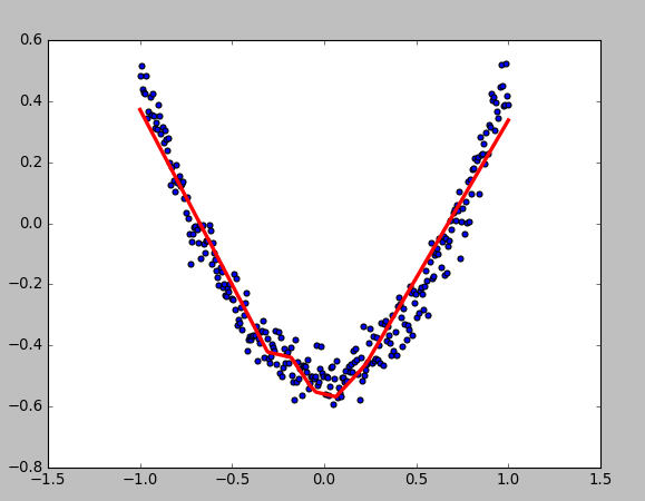
- 显示数据
fig = plt.figure()
ax = fig.add_subplot(111)
ax.scatter(x_data,y_data)
plt.ion() # 绘画之后不暂停
plt.show()
- 动态绘画
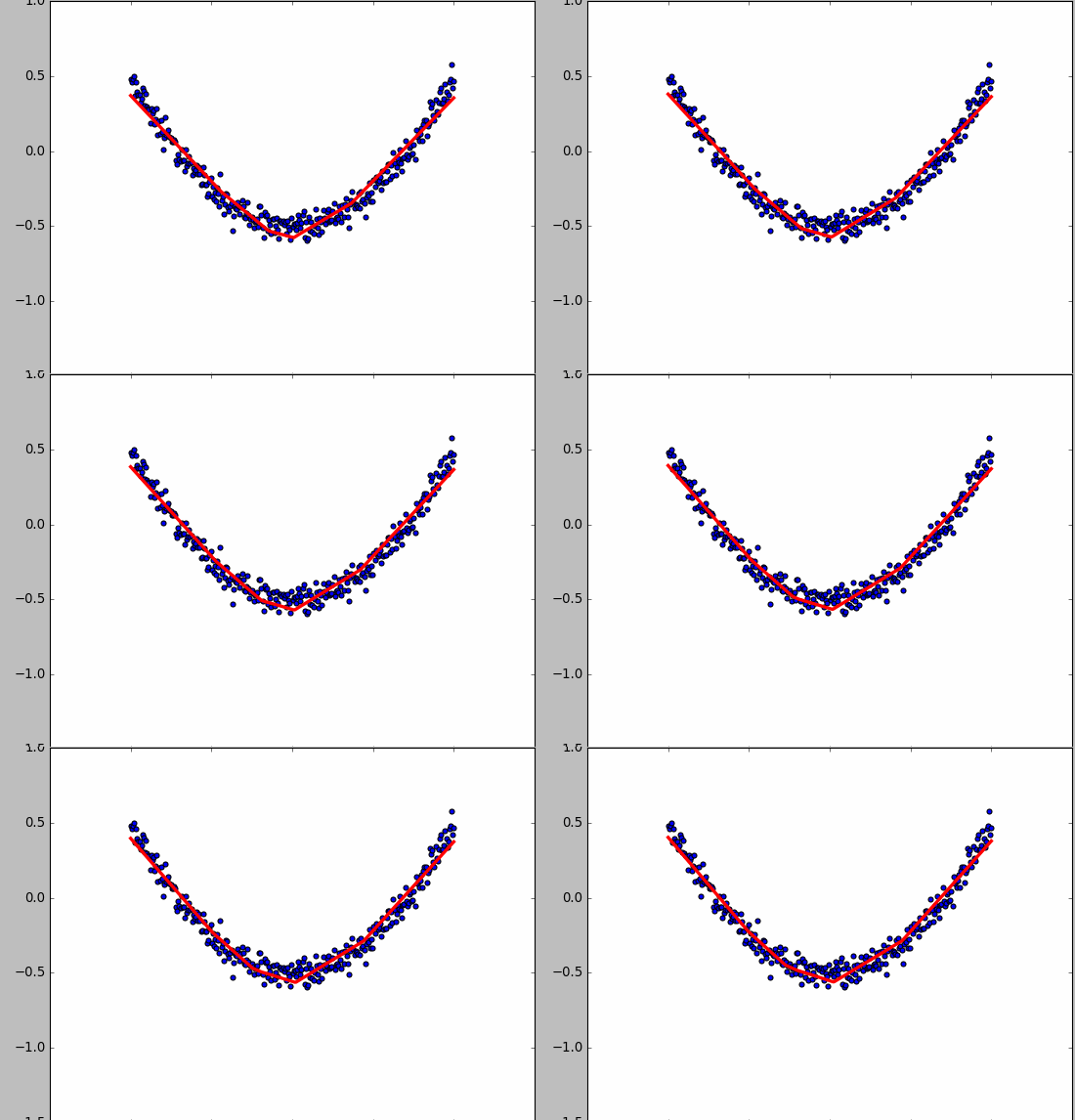
try:
ax.lines.remove(lines[0]) # 每次绘画需要移除上次绘画的结果,放在try catch里因为第一次执行没有,所以直接pass
except Exception:
pass
prediction_value = sess.run(prediction, feed_dict={xs: x_data})
# plot the prediction
lines = ax.plot(x_data, prediction_value, 'r-', lw=3) # 绘画
plt.pause(0.1) # 停0.1s
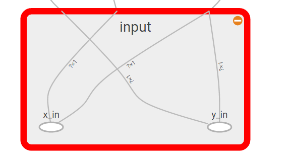
- 输入
input
with tf.name_scope('input'):
xs = tf.placeholder(tf.float32,[None,1],name='x_in') # ys = tf.placeholder(tf.float32,[None,1],name='y_in')
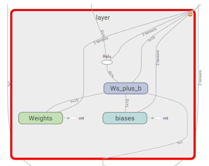
layer层
def add_layer(inputs,in_size,out_size,activation_function=None):
with tf.name_scope('layer'):
with tf.name_scope('Weights'):
Weights = tf.Variable(tf.random_normal([in_size,out_size]),name='W')
with tf.name_scope('biases'):
biases = tf.Variable(tf.zeros([1,out_size]) + 0.1,name='b')
with tf.name_scope('Ws_plus_b'):
Ws_plus_b = tf.matmul(inputs,Weights) + biases
if activation_function is None: outputs = Ws_plus_b
else: outputs = activation_function(Ws_plus_b) return outputs
loss和train
with tf.name_scope('loss'):
loss = tf.reduce_mean(tf.reduce_sum(tf.square(ys-prediction),reduction_indices=[1]))
with tf.name_scope('train'):
train = tf.train.GradientDescentOptimizer(0.1).minimize(loss)
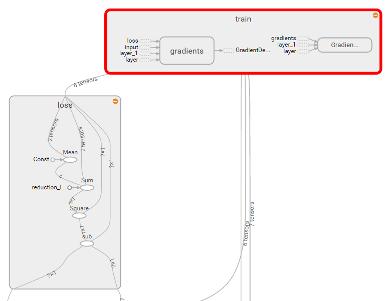
- 写入文件中
writer = tf.train.SummaryWriter("logs/", sess.graph)
- 浏览器中查看(chrome浏览器)
- 在终端输入:
tensorboard --logdir='logs/',它会给出访问地址 - 浏览器中查看即可。
tensorboard命令在安装python目录的bin目录下,可以创建一个软连接
- 可视化Weights权重和biases偏置
- 每一层起个名字
layer_name = 'layer%s'%n_layer
- tf.histogram_summary(name,value)
def add_layer(inputs,in_size,out_size,n_layer,activation_function=None):
layer_name = 'layer%s'%n_layer
with tf.name_scope(layer_name):
with tf.name_scope('Weights'):
Weights = tf.Variable(tf.random_normal([in_size,out_size]),name='W')
tf.histogram_summary(layer_name+'/weights', Weights)
with tf.name_scope('biases'):
biases = tf.Variable(tf.zeros([1,out_size]) + 0.1,name='b')
tf.histogram_summary(layer_name+'/biases',biases)
with tf.name_scope('Ws_plus_b'):
Ws_plus_b = tf.matmul(inputs,Weights) + biases
if activation_function is None: outputs = Ws_plus_b else: outputs = activation_function(Ws_plus_b) tf.histogram_summary(layer_name+'/outputs',outputs)
return outputs
- merge所有的summary
merged =tf.merge_all_summaries() - 写入文件中
writer = tf.train.SummaryWriter("logs/", sess.graph)
- 训练1000次,每50步显示一次:
for i in range(1000):
sess.run(train,feed_dict={xs:x_data,ys:y_data})
if i%50==0:
summary = sess.run(merged, feed_dict={xs: x_data, ys:y_data})
writer.add_summary(summary, i)
同样适用
tensorboard查看
可视化损失函数(代价函数)
添加:
tf.scalar_summary('loss',loss)
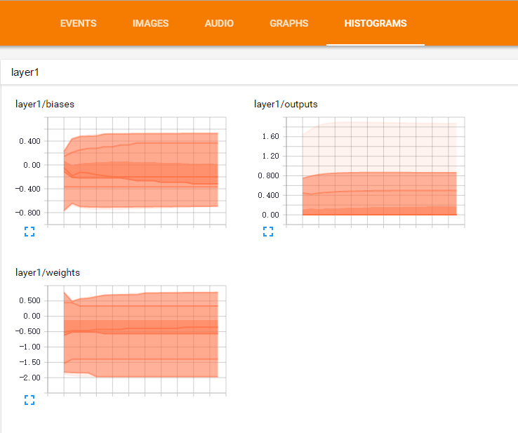
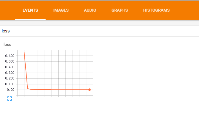
- 全部代码:
https://github.com/lawlite19/MachineLearning_TensorFlow/blob/master/Mnist_02/mnist.py - 自己的数据集,没有使用tensorflow中mnist数据集,
- 之前在机器学习中用Python实现过,地址:
https://github.com/lawlite19/MachineLearning_Python,这里使用tensorflow实现 - 神经网络只有两层
- 添加一层
'''添加一层神经网络'''
def add_layer(inputs,in_size,out_size,activation_function=None):
Weights = tf.Variable(tf.random_normal([in_size,out_size])) # 权重,in*out biases = tf.Variable(tf.zeros([1,out_size]) + 0.1) Ws_plus_b = tf.matmul(inputs,Weights) + biases # 计算权重和偏置之后的值 if activation_function is None: outputs = Ws_plus_b else: outputs = activation_function(Ws_plus_b) # 调用激励函数运算 return outputs
- 运行函数
'''运行函数'''
def NeuralNetwork():
data_digits = spio.loadmat('data_digits.mat')
X = data_digits['X']
y = data_digits['y']
m,n = X.shape
class_y = np.zeros((m,10)) # y是0,1,2,3...9,需要映射0/1形式
for i in range(10):
class_y[:,i] = np.float32(y==i).reshape(1,-1) xs = tf.placeholder(tf.float32, shape=[None,400]) # 像素是20x20=400,所以有400个feature
ys = tf.placeholder(tf.float32, shape=[None,10]) # 输出有10个
prediction = add_layer(xs, 400, 10, activation_function=tf.nn.softmax) # 两层神经网络,400x10
#prediction = add_layer(layer1, 25, 10, activation_function=tf.nn.softmax)
#loss = tf.reduce_mean(tf.reduce_sum(tf.square(ys-prediction),reduction_indices=[1]))
loss = tf.reduce_mean(-tf.reduce_sum(ys*tf.log(prediction),reduction_indices=[1])) # 定义损失函数(代价函数),
train = tf.train.GradientDescentOptimizer(learning_rate=0.5).minimize(loss) # 使用梯度下降最小化损失
init = tf.initialize_all_variables() # 初始化所有变量
sess = tf.Session() # 创建Session
sess.run(init)
for i in range(4000): # 迭代训练4000次
sess.run(train, feed_dict={xs:X,ys:class_y}) # 训练train,填入数据
if i%50==0: # 每50次输出当前的准确度
print(compute_accuracy(xs,ys,X,class_y,sess,prediction))
- 计算准确度
'''计算预测准确度''' def compute_accuracy(xs,ys,X,y,sess,prediction):
y_pre = sess.run(prediction,feed_dict={xs:X}) correct_prediction = tf.equal(tf.argmax(y_pre,1),tf.argmax(y,1)) #tf.argmax 给出某个tensor对象在某一维上的其数据最大值所在的索引值,即为对应的数字,tf.equal 来检测我们的预测是否真实标签匹配
accuracy = tf.reduce_mean(tf.cast(correct_prediction,tf.float32)) # 平均值即为准确度
result = sess.run(accuracy,feed_dict={xs:X,ys:y})
return result - 输出每一次预测的结果准确度

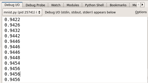
- 全部代码:
https://github.com/lawlite19/MachineLearning_TensorFlow/blob/master/Mnist_02/mnist.py - 采用TensorFlow中的mnist数据集(可以取网站下载它的数据集,http://yann.lecun.com/exdb/mnist/)
- 实现代码与上面类似,它有专门的测试集
- 随机梯度下降
SGD,每次选出100个数据进行训练
for i in range(2000):
batch_xs, batch_ys = minist.train.next_batch(100)
sess.run(train_step,feed_dict={xs:batch_xs,ys:batch_ys})
if i%50==0:
print(compute_accuracy(xs,ys,minist.test.images, minist.test.labels,sess,prediction))
- 输出每一次预测的结果准确度

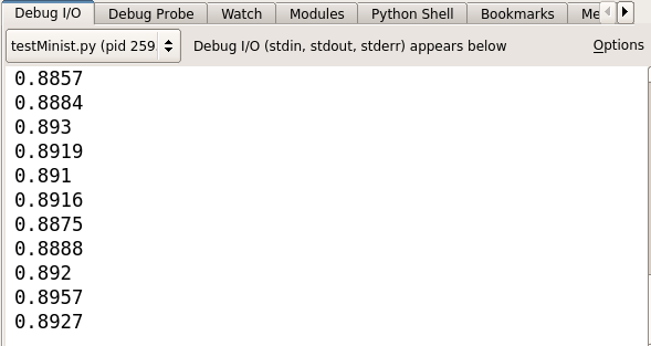
- 关于卷积神经网络CNN可以查看我的博客:http://blog.csdn.net/u013082989/article/details/53673602
- 或者github:https://github.com/lawlite19/DeepLearning_Python
- 全部代码:
https://github.com/lawlite19/MachineLearning_TensorFlow/blob/master/Mnist_03_CNN/mnist_cnn.py - 采用TensorFlow中的mnist数据集(可以取网站下载它的数据集,http://yann.lecun.com/exdb/mnist/)
- 权重和偏置初始化函数
- 权重使用的
truncated_normal进行初始化,stddev标准差定义为0.1 - 偏置初始化为常量0.1
'''权重初始化函数'''
def weight_variable(shape):
inital = tf.truncated_normal(shape, stddev=0.1) # 使用truncated_normal进行初始化
return tf.Variable(inital)
'''偏置初始化函数'''
def bias_variable(shape):
inital = tf.constant(0.1,shape=shape) # 偏置定义为常量
return tf.Variable(inital)
- 卷积函数
strides[0]和strides[3]的两个1是默认值,中间两个1代表padding时在x方向运动1步,y方向运动1步padding='SAME'代表经过卷积之后的输出图像和原图像大小一样
'''卷积函数'''
def conv2d(x,W):#x是图片的所有参数,W是此卷积层的权重
return tf.nn.conv2d(x,W,strides=[1,1,1,1],padding='SAME')#strides[0]和strides[3]的两个1是默认值,中间两个1代表padding时在x方向运动1步,y方向运动1步
- 池化函数
ksize指定池化核函数的大小- 根据池化核函数的大小定义
strides的大小
'''池化函数'''
def max_pool_2x2(x):
return tf.nn.max_pool(x,ksize=[1,2,2,1],
strides=[1,2,2,1], padding='SAME')#池化的核函数大小为2x2,因此ksize=[1,2,2,1],步长为2,因此strides=[1,2,2,1]
- 加载
mnist数据和定义placeholder - 输入数据
x_image最后一个1代表channel的数量,若是RGB3个颜色通道就定义为3 keep_prob用于dropout防止过拟合
mnist = input_data.read_data_sets('MNIST_data', one_hot=True) # 下载数据
xs = tf.placeholder(tf.float32,[None,784]) # 输入图片的大小,28x28=784
ys = tf.placeholder(tf.float32,[None,10]) # 输出0-9共10个数字
keep_prob = tf.placeholder(tf.float32) # 用于接收dropout操作的值,dropout为了防止过拟合
x_image = tf.reshape(xs,[-1,28,28,1]) #-1代表先不考虑输入的图片例子多少这个维度,后面的1是channel的数量,因为我们输入的图片是黑白的,因此channel是1,例如如果是RGB图像,那么channel就是3
- 第一层卷积和池化
- 使用ReLu激活函数
'''第一层卷积,池化'''
W_conv1 = weight_variable([5,5,1,32]) # 卷积核定义为5x5,1是输入的通道数目,32是输出的通道数目
b_conv1 = bias_variable([32]) # 每个输出通道对应一个偏置
h_conv1 = tf.nn.relu(conv2d(x_image,W_conv1)+b_conv1) # 卷积运算,并使用ReLu激活函数激活
h_pool1 = max_pool_2x2(h_conv1) # pooling操作 - 第二层卷积和池化
'''第二层卷积,池化'''
W_conv2 = weight_variable([5,5,32,64]) # 卷积核还是5x5,32个输入通道,64个输出通道
b_conv2 = bias_variable([64]) # 与输出通道一致
h_conv2 = tf.nn.relu(conv2d(h_pool1, W_conv2)+b_conv2)
h_pool2 = max_pool_2x2(h_conv2)
- 全连接第一层
'''全连接层'''
h_pool2_flat = tf.reshape(h_pool2, [-1,7*7*64]) # 将最后操作的数据展开
W_fc1 = weight_variable([7*7*64,1024]) # 下面就是定义一般神经网络的操作了,继续扩大为1024
b_fc1 = bias_variable([1024]) # 对应的偏置
h_fc1 = tf.nn.relu(tf.matmul(h_pool2_flat,W_fc1)+b_fc1) # 运算、激活(这里不是卷积运算了,就是对应相乘)
dropout防止过拟合
'''dropout'''
h_fc1_drop = tf.nn.dropout(h_fc1,keep_prob) # dropout操作
- 最后一层全连接预测,使用梯度下降优化交叉熵损失函数
- 使用softmax分类器分类
'''最后一层全连接'''
W_fc2 = weight_variable([1024,10]) # 最后一层权重初始化
b_fc2 = bias_variable([10]) # 对应偏置
prediction = tf.nn.softmax(tf.matmul(h_fc1_drop,W_fc2)+b_fc2) # 使用softmax分类器
cross_entropy = tf.reduce_mean(-tf.reduce_sum(ys*tf.log(prediction),reduction_indices=[1])) # 交叉熵损失函数来定义cost function
train_step = tf.train.AdamOptimizer(1e-3).minimize(cross_entropy) # 调用梯度下降
- 定义Session,使用
SGD训练
'''下面就是tf的一般操作,定义Session,初始化所有变量,placeholder传入值训练'''
sess = tf.Session()
sess.run(tf.initialize_all_variables())
for i in range(1000):
batch_xs, batch_ys = mnist.train.next_batch(100) # 使用SGD,每次选取100个数据训练
sess.run(train_step, feed_dict={xs: batch_xs, ys: batch_ys, keep_prob: 0.5}) # dropout值定义为0.5
if i % 50 == 0:
print compute_accuracy(xs,ys,mnist.test.images, mnist.test.labels,keep_prob,sess,prediction) # 每50次输出一下准确度
- 计算准确度函数
- 和上面的两个计算准确度的函数一致,就是多了个dropout的参数
keep_prob
- 和上面的两个计算准确度的函数一致,就是多了个dropout的参数
'''计算准确度函数'''
def compute_accuracy(xs,ys,X,y,keep_prob,sess,prediction):
y_pre = sess.run(prediction,feed_dict={xs:X,keep_prob:1.0}) # 预测,这里的keep_prob是dropout时用的,防止过拟合
correct_prediction = tf.equal(tf.argmax(y_pre,1),tf.argmax(y,1)) #tf.argmax 给出某个tensor对象在某一维上的其数据最大值所在的索引值,即为对应的数字,tf.equal 来检测我们的预测是否真实标签匹配
accuracy = tf.reduce_mean(tf.cast(correct_prediction,tf.float32)) # 平均值即为准确度
result = sess.run(accuracy,feed_dict={xs:X,ys:y,keep_prob:1.0})
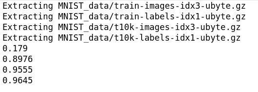
return result - 测试集上准确度

- 使用
top命令查看占用的CPU和内存,还是很消耗CPU和内存的,所以上面只输出了四次我就终止了
- 由于我在虚拟机里运行的
TensorFlow程序,分配了5G的内存,若是内存不够会报一个错误。

- 定义要保存的数据
W = tf.Variable(initial_value=[[1,2,3],[3,4,5]], name='weights', dtype=tf.float32) # 注意需要指定name和dtype
b = tf.Variable(initial_value=[1,2,3], name='biases', dtype=tf.float32)
init = tf.initialize_all_variables()
- 保存
saver = tf.train.Saver()
with tf.Session() as sess:
sess.run(init)
save_path = saver.save(sess, 'my_network/save_net.ckpt') # 保存目录,注意要在当前项目下建立my_network的目录
print ('保存到 :',save_path)
- 定义数据
W = tf.Variable(np.arange(6).reshape((2,3)), name='weights', dtype=tf.float32) # 注意与之前保存的一致
b = tf.Variable(np.arange((3)), name='biases', dtype=tf.float32)
restore提取
saver = tf.train.Saver() with tf.Session() as sess:
saver.restore(sess,'my_network/save_net.ckpt') print('weights:',sess.run(W)) # 输出一下结果
print('biases:',sess.run(b))
- 全部代码
- 使用
MNIST数据集
'''Load MNIST data and print some information'''data=input_data.read_data_sets("MNIST_data", one_hot=True)
print("Size of:")
print("\t training-set:\t\t{}".format(len(data.train.labels)))
print("\t test-set:\t\t\t{}".format(len(data.test.labels)))
print("\t validation-set:\t{}".format(len(data.validation.labels)))
print(data.test.labels[0:5])
data.test.cls=np.array([label.argmax() forlabel indata.test.labels]) # gettheactualvalueprint(data.test.cls[0:5])- 实现函数
'''define a funciton to plot 9 images'''defplot_images(images, cls_true, cls_pred=None):'''
@parameter images: the images info
@parameter cls_true: the true value of image
@parameter cls_pred: the prediction value, default is None
'''
assertlen(images) ==len(cls_true) ==9 # onlyshow9images
fig, axes = plt.subplots(nrows=3, ncols=3)
fori, ax inenumerate(axes.flat):
ax.imshow(images[i].reshape(img_shape), cmap="binary") # binary means black_white image
# show the true and pred values
ifcls_predisNone:xlabel="True: {0}".format(cls_true[i])
else:
xlabel="True: {0},Pred: {1}".format(cls_true[i],cls_pred[i])
ax.set_xlabel(xlabel)
ax.set_xticks([]) # remove the ticks
ax.set_yticks([])
plt.show()- 选择测试集中的9张图显示
'''show 9 images'''images=data.test.images[0:9]
cls_true=data.test.cls[0:9]
plot_images(images, cls_true)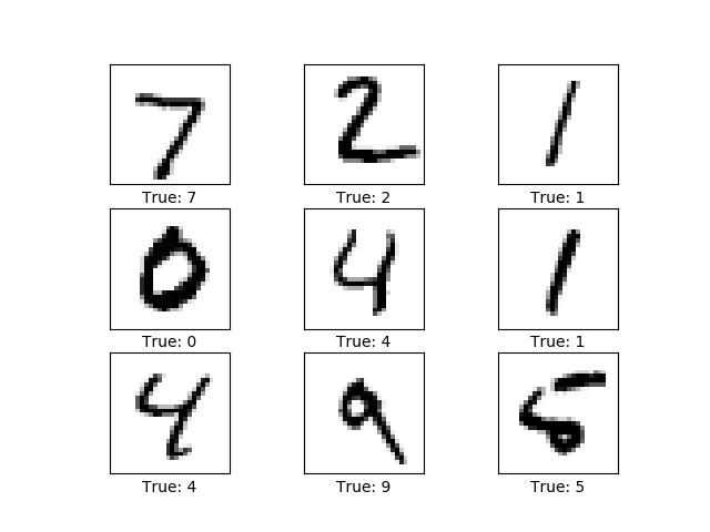
- 定义
placeholder
'''define the placeholder'''X=tf.placeholder(tf.float32, [None, img_size_flat]) # Nonemeansthearbitrarynumberoflabels, thefeaturessizeisimg_size_flaty_true=tf.placeholder(tf.float32, [None, num_classes]) # outputsizeisnum_classesy_true_cls=tf.placeholder(tf.int64, [None])- 定义
weights和biases
'''define weights and biases'''weights=tf.Variable(tf.zeros([img_size_flat, num_classes])) # img_size_flat*num_classesbiases=tf.Variable(tf.zeros([num_classes]))- 定义模型
'''define the model'''logits=tf.matmul(X,weights) +biasesy_pred=tf.nn.softmax(logits)
y_pred_cls=tf.argmax(y_pred, dimension=1)
cross_entropy=tf.nn.softmax_cross_entropy_with_logits(labels=y_true, logits=logits)
cost=tf.reduce_mean(cross_entropy)
'''define the optimizer'''optimizer=tf.train.GradientDescentOptimizer(learning_rate=0.5).minimize(cost)
- 定义求准确度
'''define the accuracy'''correct_prediction=tf.equal(y_pred_cls, y_true_cls)
accuracy=tf.reduce_mean(tf.cast(correct_prediction, tf.float32))- 定义
session
'''run the datagraph and use batch gradient descent'''session=tf.Session()
session.run(tf.global_variables_initializer())
batch_size=100'''define a function to run the optimizer'''defoptimize(num_iterations):'''
@parameter num_iterations: the traning times
'''
fori inrange(num_iterations):
x_batch, y_true_batch = data.train.next_batch(batch_size)
feed_dict_train={X: x_batch,y_true:y_true_batch}
session.run(optimizer, feed_dict=feed_dict_train)
- 代码
feed_dict_test={X: data.test.images, y_true: data.test.labels, y_true_cls: data.test.cls}'''define a function to print the accuracy'''defprint_accuracy():acc=session.run(accuracy, feed_dict=feed_dict_test)
print("Accuracy on test-set:{0:.1%}".format(acc))- 输出:
Accuracy on test-set:89.4%
- 代码
'''define a function to plot the error prediciton'''defplot_example_errors():
correct, cls_pred = session.run([correct_prediction, y_pred_cls], feed_dict=feed_dict_test) incorrect= (correct==False)
images=data.test.images[incorrect] # getthepredictionerrorimagescls_pred=cls_pred[incorrect] # getpredictionvaluecls_true=data.test.cls[incorrect] # gettruevalueplot_images(images[0:9], cls_true[0:9], cls_pred[0:9])- 输出:

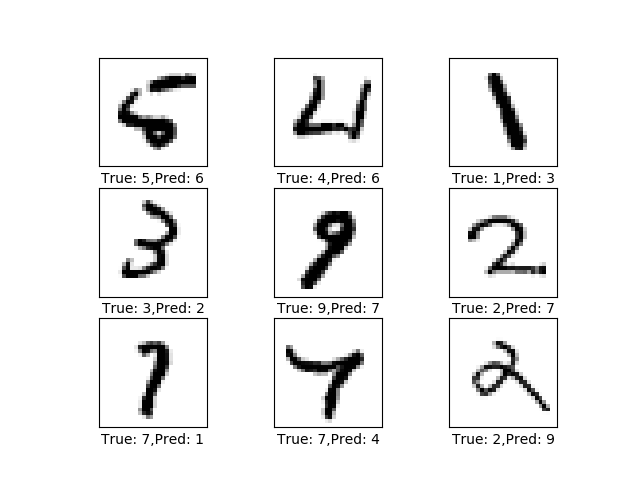
- 代码
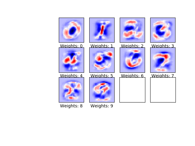
'''define a fucntion to plot weights'''defplot_weights():w=session.run(weights)
w_min=np.min(w)
w_max=np.max(w)
fig, axes = plt.subplots(3, 4)
fig.subplots_adjust(0.3, 0.3)
fori, ax inenumerate(axes.flat):ifi<10:image=w[:,i].reshape(img_shape)
ax.set_xlabel("Weights: {0}".format(i))
ax.imshow(image, vmin=w_min,vmax=w_max,cmap="seismic")
ax.set_xticks([])
ax.set_yticks([])
plt.show()- 输出:

- 代码:
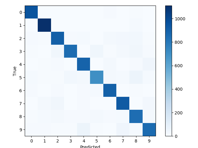
'''define a function to printand plot the confusion matrix using scikit-learn.'''defprint_confusion_martix():cls_true=data.test.cls # testsetactualvaluecls_pred=session.run(y_pred_cls, feed_dict=feed_dict_test) # testsetpredictvaluecm=confusion_matrix(y_true=cls_true,y_pred=cls_pred) # usesklearnconfusion_matrixprint(cm)
plt.imshow(cm, interpolation='nearest',cmap=plt.cm.Blues) # Plot the confusion matrix as an image.
plt.tight_layout()
plt.colorbar()
tick_marks=np.arange(num_classes)
tick_marks=np.arange(num_classes)
plt.xticks(tick_marks, range(num_classes))
plt.yticks(tick_marks, range(num_classes))
plt.xlabel('Predicted')
plt.ylabel('True') plt.show()- 输出:

- 全部代码
- 使用
MNIST数据集 - 加载数据,绘制9张图等函数与上面一致,
readme中不再写出
'''define cnn description'''filter_size1=5 # thefirstconvfiltersizeis5x5num_filters1=32 # thereare32filtersfilter_size2=5 # thesecondconvfiltersizenum_filters2=64 # thereare64filtersfc_size=1024 # fully-connectedlayer'''define a function to intialize weights'''definitialize_weights(shape):'''
@param shape:the shape of weights
'''
returntf.Variable(tf.truncated_normal(shape=shape, stddev=0.1))
'''define a function to intialize biases'''definitialize_biases(length):'''
@param length: the length of biases, which is a vector
'''
returntf.Variable(tf.constant(0.1,shape=[length]))'''define a function to do conv and pooling if used'''defconv_layer(input, num_input_channels,
filter_size,
num_output_filters,
use_pooling=True):'''
@param input: the input of previous layer's output
@param num_input_channels: input channels
@param filter_size: the weights filter size
@param num_output_filters: the output number channels
@param use_pooling:ifusepoolingoperation'''
shape= [filter_size, filter_size, num_input_channels, num_output_filters]
weights=initialize_weights(shape=shape)
biases=initialize_biases(length=num_output_filters) # oneforeachfilterlayer=tf.nn.conv2d(input=input, filter=weights, strides=[1,1,1,1], padding='SAME')
layer+=biasesifuse_pooling:layer=tf.nn.max_pool(value=layer,
ksize=[1,2,2,1],
strides=[1,2,2,1],
padding="SAME") # thekernelfunctionsizeis2x2,sotheksize=[1,2,2,1]
layer=tf.nn.relu(layer)
returnlayer, weights'''define a function to flat conv layer'''defflatten_layer(layer):'''
@param layer: the conv layer
'''
layer_shape=layer.get_shape() # gettheshapeofthelayer(layer_shape== [num_images, img_height, img_width, num_channels])
num_features=layer_shape[1:4].num_elements() # [1:4] meansthelastthreedemension, namelytheflattensizelayer_flat=tf.reshape(layer, [-1, num_features]) # reshapetoflat,-1meansdon'tcareaboutthenumberofimagesreturnlayer_flat, num_features'''define a function to do fully-connected'''deffc_layer(input, num_inputs, num_outputs, use_relu=True):'''
@param input: the input
@param num_inputs: the input size
@param num_outputs: the output size
@param use_relu:ifusereluactivationfunction'''
weights=initialize_weights(shape=[num_inputs, num_outputs])
biases=initialize_biases(num_outputs)
layer=tf.matmul(input, weights) +biasesifuse_relu:layer=tf.nn.relu(layer)
returnlayer- 定义
placeholder
'''define the placeholder'''X=tf.placeholder(tf.float32, shape=[None, img_flat_size], name="X")
X_image=tf.reshape(X, shape=[-1, img_size, img_size, num_channels]) # reshapetotheimageshapey_true=tf.placeholder(tf.float32, [None, num_classes], name="y_true")
y_true_cls=tf.argmax(y_true, axis=1)
keep_prob=tf.placeholder(tf.float32) # dropoutplaceholder- 定义卷积、dropout、和全连接
'''define the cnn model'''
layer_conv1, weights_conv1 =conv_layer(input=X_image, num_input_channels=num_channels, filter_size=filter_size1, num_output_filters=num_filters1,
use_pooling=True)
print("conv1:",layer_conv1)
layer_conv2, weights_conv2 =conv_layer(input=layer_conv1, num_input_channels=num_filters1, filter_size=filter_size2,
num_output_filters=num_filters2,
use_pooling=True)
print("conv2:",layer_conv2)
layer_flat, num_features =flatten_layer(layer_conv2) # the num_feature is 7x7x36=1764
print("flatten layer:", layer_flat) layer_fc1=fc_layer(layer_flat, num_features, fc_size, use_relu=True)
print("fully-connected layer1:", layer_fc1)
layer_drop_out=tf.nn.dropout(layer_fc1, keep_prob) # dropoutoperationlayer_fc2=fc_layer(layer_drop_out, fc_size, num_classes,use_relu=False)
print("fully-connected layer2:", layer_fc2)
y_pred=tf.nn.softmax(layer_fc2)
y_pred_cls=tf.argmax(y_pred, axis=1)
cross_entropy=tf.nn.softmax_cross_entropy_with_logits(labels=y_true, logits=layer_fc2)
cost=tf.reduce_mean(cross_entropy)
optimizer=tf.train.AdamOptimizer(learning_rate=1e-3).minimize(cost) # useAdamOptimizer优化
- 定义求准确度
'''define accuracy'''correct_prediction=tf.equal(y_true_cls, y_pred_cls)
accuracy=tf.reduce_mean(tf.cast(correct_prediction,dtype=tf.float32))- 代码:
'''define a function to run train the model with bgd'''total_iterations=0 # recordthetotaliterationsdefoptimize(num_iterations):'''
@param num_iterations: the total interations of train batch_size operation
'''
globaltotal_iterationsstart_time=time.time()
fori inrange(total_iterations,total_iterations+num_iterations):
x_batch, y_batch = data.train.next_batch(batch_size)
feed_dict={X: x_batch, y_true:y_batch, keep_prob:0.5}
session.run(optimizer, feed_dict=feed_dict)
ifi%10==0:acc=session.run(accuracy, feed_dict=feed_dict)
msg="Optimization Iteration: {0:>6}, Training Accuracy: {1:>6.1%}" # {:>6}meansthefixedwidth,{1:>6.1%}meansthefixedwidthis6andkeep1decimalplaceprint(msg.format(i+1, acc))
total_iterations+=num_iterationsend_time=time.time()
time_dif=end_time-start_timeprint("time usage:"+str(timedelta(seconds=int(round(time_dif)))))- 输出:
OptimizationIteration:651, TrainingAccuracy:99.0%OptimizationIteration:661, TrainingAccuracy:99.0%OptimizationIteration:671, TrainingAccuracy:99.0%OptimizationIteration:681, TrainingAccuracy:99.0%OptimizationIteration:691, TrainingAccuracy:99.0%OptimizationIteration:701, TrainingAccuracy:99.0%OptimizationIteration:711, TrainingAccuracy:99.0%OptimizationIteration:721, TrainingAccuracy:99.0%OptimizationIteration:731, TrainingAccuracy:99.0%OptimizationIteration:741, TrainingAccuracy:100.0%OptimizationIteration:751, TrainingAccuracy:99.0%OptimizationIteration:761, TrainingAccuracy:99.0%OptimizationIteration:771, TrainingAccuracy:97.0%OptimizationIteration:781, TrainingAccuracy:96.0%OptimizationIteration:791, TrainingAccuracy:98.0%OptimizationIteration:801, TrainingAccuracy:100.0%OptimizationIteration:811, TrainingAccuracy:100.0%OptimizationIteration:821, TrainingAccuracy:97.0%OptimizationIteration:831, TrainingAccuracy:98.0%OptimizationIteration:841, TrainingAccuracy:99.0%OptimizationIteration:851, TrainingAccuracy:99.0%OptimizationIteration:861, TrainingAccuracy:99.0%OptimizationIteration:871, TrainingAccuracy:96.0%OptimizationIteration:881, TrainingAccuracy:99.0%OptimizationIteration:891, TrainingAccuracy:99.0%OptimizationIteration:901, TrainingAccuracy:98.0%OptimizationIteration:911, TrainingAccuracy:99.0%OptimizationIteration:921, TrainingAccuracy:99.0%OptimizationIteration:931, TrainingAccuracy:99.0%OptimizationIteration:941, TrainingAccuracy:98.0%OptimizationIteration:951, TrainingAccuracy:100.0%OptimizationIteration:961, TrainingAccuracy:99.0%OptimizationIteration:971, TrainingAccuracy:98.0%OptimizationIteration:981, TrainingAccuracy:99.0%OptimizationIteration:991, TrainingAccuracy:100.0%time usage:0:07:07batch_size_test=256defprint_test_accuracy(print_error=False,print_confusion_matrix=False):'''
@param print_error: whether plot the error images
@param print_confusion_matrix: whether plot the confusion_matrix
'''
num_test=len(data.test.images) cls_pred=np.zeros(shape=num_test, dtype=np.int) # declarethecls_predi=0#predict the test set using batch_sizewhilei<num_test:j=min(i+batch_size_test, num_test)
images=data.test.images[i:j,:]
labels=data.test.labels[i:j,:]
feed_dict={X:images,y_true:labels,keep_prob:0.5}
cls_pred[i:j] = session.run(y_pred_cls,feed_dict=feed_dict)
i=jcls_true=data.test.clscorrect= (cls_true==cls_pred)
correct_sum=correct.sum() # correctpredictionsacc=float(correct_sum)/num_testmsg="Accuracy on Test-Set: {0:.1%} ({1} / {2})"print(msg.format(acc, correct_sum, num_test)) ifprint_error:plot_error_pred(cls_pred,correct)
ifprint_confusion_matrix:plot_confusin_martrix(cls_pred)- 代码:
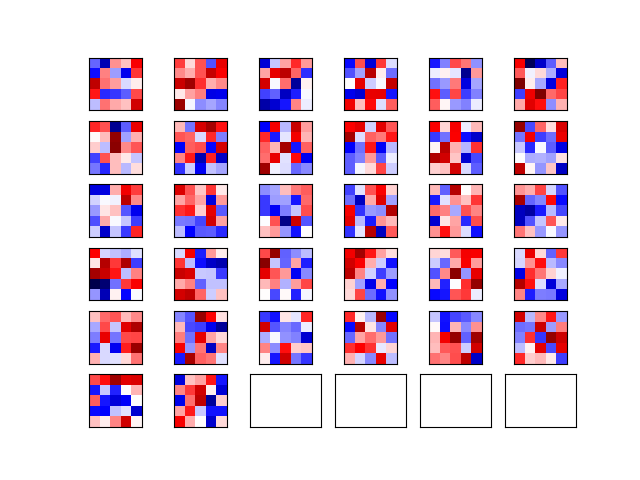
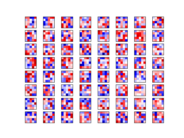
'''define a function to plot conv weights'''defplot_conv_weights(weights,input_channel=0):'''
@param weights: the conv filter weights, for example: the weights_conv1 and weights_conv2, which are 4 dimension [filter_size, filter_size, num_input_channels, num_output_filters]
@param input_channel: the input_channels
'''
w=session.run(weights)
w_min=np.min(w)
w_max=np.max(w)
num_filters=w.shape[3] # getthenumberoffiltersnum_grids=math.ceil(math.sqrt(num_filters))
fig, axes = plt.subplots(num_grids, num_grids)
fori, ax inenumerate(axes.flat):ifi<num_filters:img=w[:,:,input_channel,i] # theithweight
ax.imshow(img,vmin=w_min,vmax=w_max,interpolation="nearest",cmap='seismic')
ax.set_xticks([])
ax.set_yticks([])
plt.show()- 输出:
- 第一层:

- 第二层:

- 第一层:
- 代码:
'''define a function to plot conv output layer'''defplot_conv_layer(layer, image):'''
@param layer: the conv layer, which is also a image after conv
@param image: the image info
'''
feed_dict={X:[image]}values=session.run(layer, feed_dict=feed_dict)
num_filters=values.shape[3] # getthenumberoffiltersnum_grids=math.ceil(math.sqrt(num_filters))
fig, axes = plt.subplots(num_grids,num_grids)
fori, ax inenumerate(axes.flat):ifi<num_filters:img=values[0,:,:,i]
ax.imshow(img, interpolation="nearest",cmap="binary")
ax.set_xticks([])
ax.set_yticks([])
plt.show()- 输出:
- 第一层:

- 第二层:

- 第一层:
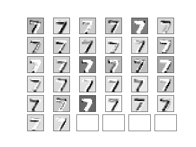
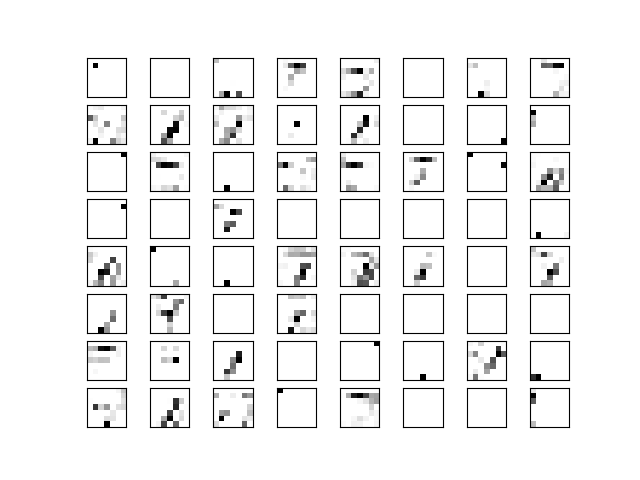
- 全部代码
- 使用
MNIST数据集 - 加载数据,绘制9张图等函数与九一致,
readme中不再写出
- 定义
placeholder,与之前的一致
'''declare the placeholder'''X=tf.placeholder(tf.float32, [None, img_flat_size], name="X")
X_img=tf.reshape(X, shape=[-1,img_size,img_size, num_channels])
y_true=tf.placeholder(tf.float32, shape=[None, num_classes], name="y_true")
y_true_cls=tf.argmax(y_true,1)- 使用
prettytensor实现CNN模型
'''define the cnn model with prettytensor'''x_pretty=pt.wrap(X_img)
withpt.defaults_scope(): # orpt.defaults_scope(activation_fn=tf.nn.relu) ifjustuseoneactivationfunction
y_pred, loss = x_pretty.\
conv2d(kernel=5, depth=16, activation_fn=tf.nn.relu, name="conv_layer1").\
max_pool(kernel=2, stride=2).\
conv2d(kernel=5, depth=36, activation_fn=tf.nn.relu, name="conv_layer2").\
max_pool(kernel=2, stride=2).\
flatten().\
fully_connected(size=128, activation_fn=tf.nn.relu, name="fc_layer1").\
softmax_classifier(num_classes=num_classes, labels=y_true)- 获取卷积核的权重(后续可视化)
'''define a function to get weights'''defget_weights_variable(layer_name):withtf.variable_scope(layer_name, reuse=True):variable=tf.get_variable("weights")
returnvariableconv1_weights=get_weights_variable("conv_layer1")
conv2_weights=get_weights_variable("conv_layer2")- 定义
optimizer训练,和之前的一样了
'''define optimizer to train'''optimizer=tf.train.AdamOptimizer().minimize(loss)
y_pred_cls=tf.argmax(y_pred,1)
correct_prediction=tf.equal(y_pred_cls, y_true_cls)
accuracy=tf.reduce_mean(tf.cast(correct_prediction, tf.float32))
session=tf.Session()
session.run(tf.global_variables_initializer())- 全部代码
- 使用
MNIST数据集 - 加载数据,绘制9张图等函数与九一致,
readme中不再写出 - CNN模型的定义和十一中的一致,
readme中不再写出
- 创建saver,和保存的目录
'''define a Saver to save the network'''saver=tf.train.Saver()
save_dir="checkpoints/"ifnotos.path.exists(save_dir):
os.makedirs(save_dir)
save_path=os.path.join(save_dir, 'best_validation')- 保存session,对应到下面2中的Early Stopping,将最好的模型保存
saver.save(sess=session, save_path=save_path)'''declear the train info'''train_batch_size=64best_validation_accuracy=0.0last_improvement=0require_improvement_iterations=1000total_iterations=0'''define a function to optimize the optimizer'''defoptimize(num_iterations):globaltotal_iterationsglobalbest_validation_accuracygloballast_improvementstart_time=time.time()
fori inrange(num_iterations):total_iterations+=1
X_batch, y_true_batch = data.train.next_batch(train_batch_size)
feed_dict_train={X: X_batch,
y_true: y_true_batch}
session.run(optimizer, feed_dict=feed_dict_train)
if (total_iterations%100==0) or (i==num_iterations-1):acc_train=session.run(accuracy, feed_dict=feed_dict_train)
acc_validation, _ =validation_accuracy()
ifacc_validation>best_validation_accuracy:best_validation_accuracy=acc_validationlast_improvement=total_iterations
saver.save(sess=session, save_path=save_path)
improved_str="*"else:
improved_str=""msg="Iter: {0:>6}, Train_batch accuracy:{1:>6.1%}, validation acc:{2:>6.1%} {3}"print(msg.format(i+1, acc_train, acc_validation, improved_str))
iftotal_iterations-last_improvement>require_improvement_iterations:print('No improvement found in a while, stop running')
breakend_time=time.time()
time_diff=end_time-start_timeprint("Time usage:"+str(timedelta(seconds=int(round(time_diff)))))- 调用
optimize(10000)输出信息
Iter: 5100, Train_batchaccuracy:100.0%, validationacc:98.8%*Iter: 5200, Train_batchaccuracy:100.0%, validationacc:98.3%Iter: 5300, Train_batchaccuracy:100.0%, validationacc:98.7%Iter: 5400, Train_batchaccuracy:98.4%, validationacc:98.6%Iter: 5500, Train_batchaccuracy:98.4%, validationacc:98.6%Iter: 5600, Train_batchaccuracy:100.0%, validationacc:98.7%Iter: 5700, Train_batchaccuracy:96.9%, validationacc:98.9%*Iter: 5800, Train_batchaccuracy:100.0%, validationacc:98.6%Iter: 5900, Train_batchaccuracy:100.0%, validationacc:98.6%Iter: 6000, Train_batchaccuracy:98.4%, validationacc:98.7%Iter: 6100, Train_batchaccuracy:100.0%, validationacc:98.7%Iter: 6200, Train_batchaccuracy:100.0%, validationacc:98.7%Iter: 6300, Train_batchaccuracy:98.4%, validationacc:98.8%Iter: 6400, Train_batchaccuracy:98.4%, validationacc:98.8%Iter: 6500, Train_batchaccuracy:100.0%, validationacc:98.7%Iter: 6600, Train_batchaccuracy:100.0%, validationacc:98.7%Iter: 6700, Train_batchaccuracy:100.0%, validationacc:98.8%Noimprovementfound inawhile, stoprunningTimeusage:0:18:43可以看到最后10次输出(每100次输出一次)在验证集上准确度都没有提高,停止执行
- 因为需要预测测试集和验证集,这里参数指定需要的images
'''define a function to predict using batch'''batch_size_predict=256defpredict_cls(images, labels, cls_true):num_images=len(images)
cls_pred=np.zeros(shape=num_images, dtype=np.int)
i=0whilei<num_images:j=min(i+batch_size_predict, num_images)
feed_dict={X: images[i:j,:],
y_true: labels[i:j,:]}
cls_pred[i:j] = session.run(y_pred_cls, feed_dict=feed_dict)
i=jcorrect= (cls_true==cls_pred)
returncorrect, cls_pred- 测试集和验证集直接调用即可
defpredict_cls_test():returnpredict_cls(data.test.images, data.test.labels, data.test.cls)
defpredict_cls_validation():returnpredict_cls(data.validation.images, data.validation.labels, data.validation.cls)- 计算验证集准确率(上面optimize函数中需要用到)
'''calculate the acc'''defcls_accuracy(correct):correct_sum=correct.sum()
acc=float(correct_sum)/len(correct)
returnacc, correct_sum'''define a function to calculate the validation acc'''defvalidation_accuracy():
correct, _ =predict_cls_validation()
returncls_accuracy(correct)- 计算测试集准确率,并且输出错误的预测和confusion matrix
'''define a function to calculate test acc'''defprint_test_accuracy(show_example_errors=False,
show_confusion_matrix=False):
correct, cls_pred =predict_cls_test()
acc, num_correct =cls_accuracy(correct)
num_images=len(correct)
msg="Accuracy on Test-Set: {0:.1%} ({1} / {2})"print(msg.format(acc, num_correct, num_images))
# Plot some examples of mis-classifications, ifdesired.
ifshow_example_errors:print("Example errors:")
plot_example_errors(cls_pred=cls_pred, correct=correct)
# Plot the confusion matrix, ifdesired.
ifshow_confusion_matrix:print("Confusion Matrix:")
plot_confusion_matrix(cls_pred=cls_pred) - 全部代码
- 使用
MNIST数据集 - 一些方法和之前的一致,不在给出
- 其中训练了多个CNN 模型,然后取预测的平均值作为最后的预测结果
- 主要是希望训练时数据集有些变换,否则都是一样的数据去训练了,最后再融合意义不大
'''将training set和validation set合并,并重新划分'''combine_images=np.concatenate([data.train.images, data.validation.images], axis=0)
combine_labels=np.concatenate([data.train.labels, data.validation.labels], axis=0)
print("合并后图片:", combine_images.shape)
print("合并后label:", combine_labels.shape)
combined_size=combine_labels.shape[0]
train_size=int(0.8*combined_size)
validation_size=combined_size-train_size'''函数:将合并后的重新随机划分'''defrandom_training_set():idx=np.random.permutation(combined_size) # 将0-combined_size数字随机排列
idx_train=idx[0:train_size]
idx_validation=idx[train_size:]
x_train=combine_images[idx_train, :]
y_train=combine_labels[idx_train, :]
x_validation=combine_images[idx_validation, :]
y_validation=combine_images[idx_validation, :]
returnx_train, y_train, x_validation, y_validation- 加载训练好的模型,并输出每个模型在测试集的预测结果等
defensemble_predictions():pred_labels= []
test_accuracies= []
validation_accuracies= []
fori inrange(num_networks):
saver.restore(sess=session, save_path=get_save_path(i))
test_acc=test_accuracy()
test_accuracies.append(test_acc)
validation_acc=validation_accuracy()
validation_accuracies.append(validation_acc)
msg="网络:{0},验证集:{1:.4f},测试集{2:.4f}"print(msg.format(i, validation_acc, test_acc))
pred=predict_labels(data.test.images)
pred_labels.append(pred)
returnnp.array(pred_labels),\
np.array(test_accuracies),\
np.array(validation_accuracies)- 调用
pred_labels, test_accuracies, val_accuracies = ensemble_predictions() - 取均值:
ensemble_pred_labels = np.mean(pred_labels, axis=0) - 融合后的真实结果:
ensemble_cls_pred = np.argmax(ensemble_pred_labels, axis=1) - 其他一些信息:
ensemble_correct= (ensemble_cls_pred==data.test.cls)
ensemble_incorrect=np.logical_not(ensemble_correct)
print(test_accuracies)
best_net=np.argmax(test_accuracies)
print(best_net)
print(test_accuracies[best_net])
best_net_pred_labels=pred_labels[best_net, :, :]
best_net_cls_pred=np.argmax(best_net_pred_labels, axis=1)
best_net_correct= (best_net_cls_pred==data.test.cls)
best_net_incorrect=np.logical_not(best_net_correct)
print("融合后预测对的:", np.sum(ensemble_correct))
print("单个最好模型预测对的", np.sum(best_net_correct))
ensemble_better=np.logical_and(best_net_incorrect, ensemble_correct) # 融合之后好于单个的个数
print(ensemble_better.sum())
best_net_better=np.logical_and(best_net_correct, ensemble_incorrect) # 单个好于融合之后的个数
print(best_net_better.sum())- 全部代码
- 使用
CIFAR-10数据集 - 创建了两个网络,一个用于训练,一个用于测试,测试使用的是训练好的权重参数,所以用到参数重用
- 网络结构

- 导入包:
- 这是别人实现好的下载和处理
cifar-10数据集的diamante
- 这是别人实现好的下载和处理
importcifar10from cifar10 import img_size, num_channels, num_classes- 输出一些数据集信息
'''下载cifar10数据集, 大概163M'''
cifar10.maybe_download_and_extract()
'''加载数据集'''
images_train, cls_train, labels_train = cifar10.load_training_data()
images_test, cls_test, labels_test = cifar10.load_test_data()
'''打印一些信息'''class_names=cifar10.load_class_names()
print(class_names)
print("Size of:")
print("training set:\t\t{}".format(len(images_train)))
print("test set:\t\t\t{}".format(len(images_test)))- 显示9张图片函数
- 相比之前的,加入了
smooth
- 相比之前的,加入了
'''显示9张图片函数'''defplot_images(images, cls_true, cls_pred=None, smooth=True): # smooth是否平滑显示
assertlen(images) ==len(cls_true) ==9
fig, axes = plt.subplots(3,3)
fori, ax inenumerate(axes.flat):ifsmooth:interpolation='spline16'else:
interpolation='nearest'
ax.imshow(images[i, :, :, :], interpolation=interpolation)
cls_true_name=class_names[cls_true[i]]
ifcls_predisNone:xlabel="True:{0}".format(cls_true_name)
else:
cls_pred_name=class_names[cls_pred[i]]
xlabel="True:{0}, Pred:{1}".format(cls_true_name, cls_pred_name)
ax.set_xlabel(xlabel)
ax.set_xticks([])
ax.set_yticks([])
plt.show()X=tf.placeholder(tf.float32, shape=[None, img_size, img_size, num_channels], name="X")
y_true=tf.placeholder(tf.float32, shape=[None, num_classes], name="y")
y_true_cls=tf.argmax(y_true, axis=1)- 单张图片处理
- 原图是
32*32像素的,裁剪成24*24像素的 - 如果是训练集进行一些裁剪,翻转,饱和度等处理
- 如果是测试集,只进行简单的裁剪处理
- 这也是为什么使用
variable_scope定义两个网络
- 原图是
'''单个图片预处理, 测试集只需要裁剪就行了'''defpre_process_image(image, training):iftraining:image=tf.random_crop(image, size=[img_size_cropped, img_size_cropped, num_channels]) # 裁剪
image=tf.image.random_flip_left_right(image) # 左右翻转
image=tf.image.random_hue(image, max_delta=0.05) # 色调调整
image=tf.image.random_brightness(image, max_delta=0.2) # 曝光
image=tf.image.random_saturation(image, lower=0.0, upper=2.0) # 饱和度
'''上面的调整可能pixel值超过[0, 1], 所以约束一下'''image=tf.minimum(image, 1.0)
image=tf.maximum(image, 0.0)
else:
image=tf.image.resize_image_with_crop_or_pad(image, target_height=img_size_cropped, target_width=img_size_cropped)
returnimage- 多张图片处理
- 因为训练和测试是都是使用
batch的方式 - 调用上面处理单张图片的函数
- tf.map_fn(fn, elems)函数,前面一般是
lambda函数,后面是所有的数据
'''调用上面的函数,处理多个图片images'''defpre_process(images, training):images=tf.map_fn(lambdaimage:pre_process_image(image, training), images) # tf.map_fn()使用lambda函数
returnimages- 定义主网络图
- 使用
prettytensor - 分为
training和test两个阶段
- 使用
'''定义主网络函数'''defmain_network(images, training):x_pretty=pt.wrap(images)
iftraining:phase=pt.Phase.trainelse:
phase=pt.Phase.inferwithpt.defaults_scope(activation_fn=tf.nn.relu, phase=phase):
y_pred, loss = x_pretty.\
conv2d(kernel=5, depth=64, name="layer_conv1", batch_normalize=True).\
max_pool(kernel=2, stride=2).\
conv2d(kernel=5, depth=64, name="layer_conv2").\
max_pool(kernel=2, stride=2).\
flatten().\
fully_connected(size=256, name="layer_fc1").\
fully_connected(size=128, name="layer_fc2").\
softmax_classifier(num_classes, labels=y_true)
returny_pred, loss- 创建所有网络,包含预处理图片和主网络
- 需要使用variable_scope, 测试阶段需要
reuse训练阶段的参数
- 需要使用variable_scope, 测试阶段需要
'''创建所有网络, 包含预处理和主网络,'''defcreate_network(training):
# 使用variable_scope可以重复使用定义的变量,训练时创建新的,测试时重复使用
withtf.variable_scope("network", reuse=nottraining):images=Ximages=pre_process(images=images, training=training)
y_pred, loss =main_network(images=images, training=training)
returny_pred, loss- 创建训练阶段网络
- 定义一个
global_step记录训练的次数,下面会将其保存到checkpoint,trainable为False就不会训练改变
- 定义一个
'''训练阶段网络创建'''global_step=tf.Variable(initial_value=0, name="global_step",
trainable=False) # trainable 在训练阶段不会改变
_, loss =create_network(training=True)
optimizer=tf.train.AdamOptimizer(learning_rate=0.0001).minimize(loss, global_step)
- 定义测试阶段网络
- 同时定义准确率
'''测试阶段网络创建'''
y_pred, _ =create_network(training=False)
y_pred_cls=tf.argmax(y_pred, dimension=1)
correct_prediction=tf.equal(y_pred_cls, y_true_cls)
accuracy=tf.reduce_mean(tf.cast(correct_prediction, tf.float32))
- 获取权重变量
defget_weights_variable(layer_name):withtf.variable_scope("network/"+layer_name, reuse=True):variable=tf.get_variable("weights")
returnvariableweights_conv1=get_weights_variable("layer_conv1")
weights_conv2=get_weights_variable("layer_conv2")- 获取每层的输出变量
defget_layer_output(layer_name):tensor_name="network/"+layer_name+"/Relu:0"tensor=tf.get_default_graph().get_tensor_by_name(tensor_name)
returntensoroutput_conv1=get_layer_output("layer_conv1")
output_conv2=get_layer_output("layer_conv2")- 因为第一次不会加载,所以放到
try中判断
'''执行tensorflow graph'''session=tf.Session()
save_dir="checkpoints/"ifnotos.path.exists(save_dir):
os.makedirs(save_dir)
save_path=os.path.join(save_dir, 'cifat10_cnn')
'''尝试存储最新的checkpoint, 可能会失败,比如第一次运行checkpoint不存在等'''try:
print("开始存储最新的存储...")
last_chk_path=tf.train.latest_checkpoint(save_dir)
saver.restore(session, save_path=last_chk_path)
print("存储点来自:", last_chk_path)
except:
print("存储错误, 初始化变量")
session.run(tf.global_variables_initializer())- 获取
batch
'''SGD'''train_batch_size=64defrandom_batch():num_images=len(images_train)
idx=np.random.choice(num_images, size=train_batch_size, replace=False)
x_batch=images_train[idx, :, :, :]
y_batch=labels_train[idx, :]
returnx_batch, y_batch- 训练网络
- 每1000次保存一下
checkpoint - 因为上面会
restored已经保存训练的网络,同时也保存了训练的次数,所以可以接着训练
- 每1000次保存一下
defoptimize(num_iterations):start_time=time.time()
fori inrange(num_iterations):
x_batch, y_batch =random_batch()
feed_dict_train={X: x_batch, y_true:y_batch}
i_global, _ = session.run([global_step, optimizer], feed_dict=feed_dict_train)
if (i_global%100==0) or (i==num_iterations-1):batch_acc=session.run(accuracy, feed_dict=feed_dict_train)
msg="global step: {0:>6}, training batch accuracy: {1:>6.1%}"print(msg.format(i_global, batch_acc))
if(i_global%1000==0) or (i==num_iterations-1):
saver.save(session, save_path=save_path,
global_step=global_step)
print("保存checkpoint")
end_time=time.time()
time_diff=end_time-start_timeprint("耗时:", str(timedelta(seconds=int(round(time_diff)))))- 全部代码
- 使用训练好的
inception model,因为模型很复杂,一般的电脑运行不起来的。 - 网络结构
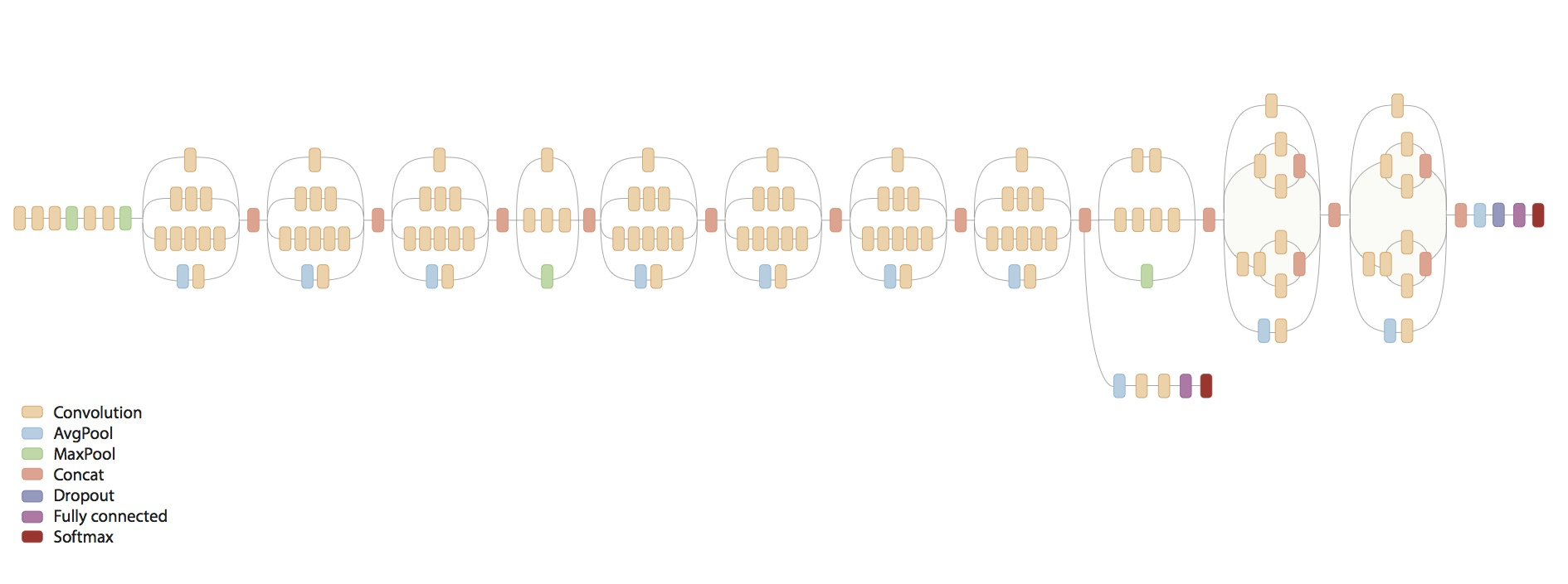
- 因为是预训练好的模型,所以无需我们定义结构了
- 导入包
- 这里
inception是别人实现好的下载的代码
- 这里
importnumpyasnpimporttensorflowastffrom matplotlib import pyplot as pltimportinception # 第三方类加载inceptionmodelimportos- 下载和加载模型
'''下载和加载inception model'''
inception.maybe_download()
model=inception.Inception()- 预测和显示图片函数
'''预测和显示图片'''defclassify(image_path):
plt.imshow(plt.imread(image_path))
plt.show()
pred=model.classify(image_path=image_path)
model.print_scores(pred=pred, k=10, only_first_name=True)- 显示调整后的图片
- 因为
inception model要求输入图片为299*299像素的,所以它会resize成这个大小然后作为输入
- 因为
'''显示处理后图片的样式'''defplot_resized_image(image_path):resized_image=model.get_resized_image(image_path)
plt.imshow(resized_image, interpolation='nearest')
plt.show()
plot_resized_image(image_path)- 全部代码
- 网络结构还是使用上一节的
inception model, 去掉最后的全连接层,然后重新构建全连接层进行训练- 因为
inception model是训练好的,前面的卷积层用于捕捉特征, 而后面的全连接层可用于分类,所以我们训练全连接层即可
- 因为
- 因为要计算每张图片的
transfer values,所以使用一个cache缓存transfer-values,第一次计算完成后,后面重新运行直接读取存储的结果,这样比较节省时间transfer values是inception model在Softmax层前一层的值cifar-10数据集, 我放在实验室电脑上运行了几个小时才得到transfer values,还是比较慢的
- 总之最后相当于训练下面的神经网络,对应的
transfer-values作为输入
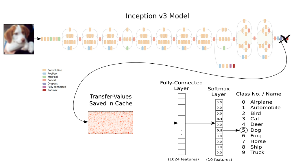
- 导入包
importnumpyasnpimporttensorflowastfimportprettytensorasptfrom matplotlib import pyplot as pltimporttimefrom datetime import timedeltaimportosimportinception # 第三方下载inceptionmodel的代码
from inception import transfer_values_cache # cacheimportcifar10 # 也是第三方的库,下载cifar-10数据集
from cifar10 import num_classes- 下载
cifar-10数据集
'''下载cifar-10数据集'''
cifar10.maybe_download_and_extract()
class_names=cifar10.load_class_names()
print("所有类别是:",class_names)
'''训练和测试集'''
images_train, cls_train, labels_train = cifar10.load_training_data()
images_test, cls_test, labels_test = cifar10.load_test_data()
- 下载和加载
inception model
'''下载inception model'''
inception.maybe_download()
model=inception.Inception()- 计算
cifar-10训练集和测试集在inception model上的transfer values- 因为计算非常耗时,这里第一次运行存储到本地,以后再运行直接读取即可
transfer values的shape是(dataset size, 2048),因为是softmax层的前一层
'''训练和测试的cache的路径'''file_path_cache_train=os.path.join(cifar10.data_path, 'inception_cifar10_train.pkl')
file_path_cache_test=os.path.join(cifar10.data_path, 'inception_cifar10_test.pkl')
print('处理训练集上的transfer-values.......... ')
image_scaled=images_train*255.0 # cifar-10的pixel是0-1的, shape=(50000, 32, 32, 3)
transfer_values_train=transfer_values_cache(cache_path=file_path_cache_train,
images=image_scaled, model=model) # shape=(50000, 2048)
print('处理测试集上的transfer-values.......... ')
images_scaled=images_test*255.0transfer_values_test=transfer_values_cache(cache_path=file_path_cache_test,
model=model,
images=images_scaled)
print("transfer_values_train: ",transfer_values_train.shape)
print("transfer_values_test: ",transfer_values_test.shape)
- 可视化一张图片对应的
transfer values
'''显示transfer values'''defplot_transfer_values(i):print("输入图片:")
plt.imshow(images_test[i], interpolation='nearest')
plt.show()
print('transfer values --> 此图片在inception model上')
img=transfer_values_test[i]
img=img.reshape((32, 64))
plt.imshow(img, interpolation='nearest', cmap='Reds')
plt.show()
plot_transfer_values(16)- 将数据降到2维,可视化,因为
transfer values是已经捕捉到的特征,所以可视化应该是可以隐约看到不同类别的数据是有区别的 - 取
3000个数据观察(因为PCA也是比较耗时的)
'''使用PCA分析transfer values'''from sklearn.decomposition import PCApca=PCA(n_components=2)
transfer_values=transfer_values_train[0:3000] # 取3000个,大的话计算量太大
cls=cls_train[0:3000]
print(transfer_values.shape)
transfer_values_reduced=pca.fit_transform(transfer_values)
print(transfer_values_reduced.shape)- 可视化降维后的数据
## 显示降维后的transfer values
defplot_scatter(values, cls):from matplotlib import cm as cmcmap=cm.rainbow(np.linspace(0.0, 1.0, num_classes))
colors=cmap[cls]
x=values[:, 0]
y=values[:, 1]
plt.scatter(x, y, color=colors)
plt.show()
plot_scatter(transfer_values_reduced, cls)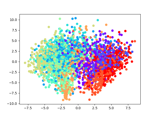
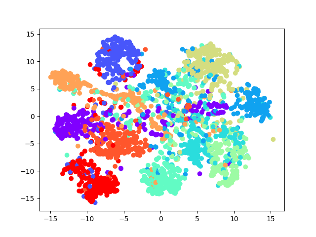
- 因为
t-SNE运行非常慢,所以这里先用PCA将到50维
from sklearn.manifold import TSNEpca=PCA(n_components=50)
transfer_values_50d=pca.fit_transform(transfer_values)
tsne=TSNE(n_components=2)
transfer_values_reduced=tsne.fit_transform(transfer_values_50d)
print("最终降维后:", transfer_values_reduced.shape)
plot_scatter(transfer_values_reduced, cls)- 数据区分还是比较明显的

- 使用
prettytensor创建一个全连接层,使用softmax作为分类
'''创建网络'''transfer_len=model.transfer_len # 获取transfervalues的大小,这里是2048x=tf.placeholder(tf.float32, shape=[None, transfer_len], name="x")
y_true=tf.placeholder(tf.float32, shape=[None, num_classes], name="y")
y_true_cls=tf.argmax(y_true, axis=1)
x_pretty=pt.wrap(x)
withpt.defaults_scope(activation_fn=tf.nn.relu):
y_pred, loss = x_pretty.\
fully_connected(1024, name="layer_fc1").\
softmax_classifier(num_classes, labels=y_true)- 优化器
'''优化器'''global_step=tf.Variable(initial_value=0, name="global_step", trainable=False)
optimizer=tf.train.AdamOptimizer(0.0001).minimize(loss, global_step)
- 准确度
'''accuracy'''y_pred_cls=tf.argmax(y_pred, axis=1)
correct_prediction=tf.equal(y_pred_cls, y_true_cls)
accuracy=tf.reduce_mean(tf.cast(correct_prediction, tf.float32))
SGD训练
'''SGD 训练'''session=tf.Session()
session.run(tf.initialize_all_variables())
train_batch_size=64defrandom_batch():num_images=len(images_train)
idx=np.random.choice(num_images, size=train_batch_size,
replace=False)
x_batch=transfer_values_train[idx]
y_batch=labels_train[idx]
returnx_batch, y_batchdefoptimize(num_iterations):start_time=time.time()
fori inrange(num_iterations):
x_batch, y_true_batch =random_batch()
feed_dict_train={x: x_batch,
y_true: y_true_batch}
i_global, _ = session.run([global_step, optimizer], feed_dict=feed_dict_train)
if (i_global%100==0) or (i==num_iterations-1):batch_acc=session.run(accuracy, feed_dict=feed_dict_train)
msg="Global Step: {0:>6}, Training Batch Accuracy: {1:>6.1%}"print(msg.format(i_global, batch_acc)) end_time=time.time()
time_diff=end_time-start_timeprint("耗时:", str(timedelta(seconds=int(round(time_diff)))))
- 使用
batch size预测测试集数据
'''batch 预测'''batch_size=256defpredict_cls(transfer_values, labels, cls_true):num_images=len(images_test)
cls_pred=np.zeros(shape=num_images, dtype=np.int)
i=0whilei<num_images:j=min(i+batch_size, num_images)
feed_dict={x: transfer_values[i:j],
y_true: labels[i:j]}
cls_pred[i:j] = session.run(y_pred_cls, feed_dict=feed_dict)
i=jcorrect= (cls_true==cls_pred)
returncorrect, cls_pred- 开启新篇章,以下内容为
RNN相关内容 - 关于
RNN的基本内容可以查看我的博客:点击查看
- 关于
RNN的基本内容参考我的博客:点击查看 - 使用
MNIST数据集,全部代码:点击查看 - 为什么可以使用
RNN来进行分类,我们可以认为像素是有关联的 - 图片的大小是
28x28的,每一行看作一个输入,共有28列,所以n_steps=28看完一张图片 - 所以输入的维度是
(batch_size, n_steps, n_inputs),输出就是(batch_size, n_classes)
- 加载数据,声明超参数
state_size是cell中的神经元个数n_steps截断梯度的步数,也就是学习多少步的依赖
print("tensorflow版本", tf.__version__)
'''读取数据'''mnist=input_data.read_data_sets('MNIST_data', one_hot=True)
print("size of")
print('--training set:\t\t{}'.format(len(mnist.train.labels)))
print('--test set:\t\t\t{}'.format(len(mnist.test.labels)))
print('--validation set:\t{}'.format(len(mnist.validation.labels)))
'''定义超参数'''learning_rate=0.001batch_size=128n_inputs=28n_steps=28state_size=128n_classes=10- 定义输入
placeholder和权重,偏置- 这里的输入权重和
biases是不用定义的,因为cell中会计算
- 这里的输入权重和
'''定义placehoder和初始化weights和biases'''x=tf.placeholder(tf.float32, [batch_size, n_steps, n_inputs], name='x')
y=tf.placeholder(tf.float32, [batch_size, n_classes], name='y')
weights={
# (28, 128)
#'in': tf.Variable(initial_value=tf.random_normal([n_inputs, state_size])),
# (128, 10)
'out': tf.Variable(tf.random_normal(shape=[state_size, n_classes], mean=0.0, stddev=1.0, dtype=tf.float32, seed=None, name=None))
}biases={
# (128, )
#'in': tf.Variable(initial_value=tf.constant(0.1,shape=[state_size,]), trainable=True, collections=None, #validate_shape=True, #caching_device=None, name=None, #variable_def=None, dtype=None, #expected_shape=None, #import_scope=None),
# (10, )
'out': tf.Variable(initial_value=tf.constant(0.1, shape=[n_classes, ]), trainable=True, collections=None, validate_shape=True, caching_device=None, name=None, variable_def=None, dtype=None, expected_shape=None, import_scope=None)
}- RNN的cell
- 使用
LSTM和dynamic_rnn的方式,关于dynamic_rnn不了解的还是请看我的博客 - 返回
rnn的输出 - 经过
n_steps=28遍历一张图片之后得到预测值,所以最后只需要最后一个的输出final_state来做最后的预测final_state[1]就是LSTM的h state,就是对应的输出
- 使用
'''定义RNN 结构'''defRNN(X, weights, biases):'''这里输入X 不用再做权重的运算,cell中会自动运算(_linear函数), 做了运算也没有实际意义,因为LSTM的cell输入的流向有多个'''
# 原始的 X 是 3 维数据, 我们需要把它变成 2 维数据才能使用 weights 的矩阵乘法
# X ==> (128 batch_size * 28 steps, 28 inputs)
#X = tf.reshape(X, [-1, n_inputs])#X_in = tf.matmul(X, weights['in']) + biases['in']
# 再换回3维
# X_in ==> (128 batches, 28 steps, 128 hidden)
#X_in = tf.reshape(X_in, shape=[-1, n_steps, state_size])'''cell中的计算方式1'''cell=tf.nn.rnn_cell.BasicLSTMCell(num_units=state_size)
init_state=cell.zero_state(batch_size, dtype=tf.float32)
rnn_outputs, final_state = tf.nn.dynamic_rnn(cell=cell,
inputs=X,
initial_state=init_state,
time_major=False)
results=tf.matmul(final_state[1], weights['out']) +biases['out']
returnresults- 预测,损失和优化器
prediction=RNN(x, weights, biases)
losses=tf.reduce_mean(tf.nn.softmax_cross_entropy_with_logits(logits=prediction,
labels=y))
train_step=tf.train.AdamOptimizer(learning_rate).minimize(losses)
prediction_cls=tf.argmax(prediction, axis=1)
correct_pred=tf.equal(prediction_cls, tf.argmax(y, 1))
accuracy=tf.reduce_mean(tf.cast(correct_pred, tf.float32))
- 训练
defoptimize(n_epochs):'''训练RNN'''withtf.Session() assess:
sess.run(tf.global_variables_initializer())
fori inrange(n_epochs):
batch_x, batch_y = mnist.train.next_batch(batch_size)
batch_x=batch_x.reshape([batch_size, n_steps, n_inputs])
feed_dict={x: batch_x, y:batch_y}
sess.run(train_step, feed_dict=feed_dict)
ifi%50==0:print("epoch: {0}, accuracy:{1}".format(i, sess.run(accuracy, feed_dict=feed_dict)))- 简单的在测试集上的准确率
epoch: 0, accuracy:0.1796875epoch: 50, accuracy:0.7109375epoch: 100, accuracy:0.828125epoch: 150, accuracy:0.8359375epoch: 200, accuracy:0.8984375epoch: 250, accuracy:0.9296875epoch: 300, accuracy:0.9375epoch: 350, accuracy:0.921875epoch: 400, accuracy:0.9609375epoch: 450, accuracy:0.953125epoch: 500, accuracy:0.921875epoch: 550, accuracy:0.9296875epoch: 600, accuracy:0.9609375epoch: 650, accuracy:0.9375epoch: 700, accuracy:0.9765625epoch: 750, accuracy:0.96875epoch: 800, accuracy:0.9375epoch: 850, accuracy:0.9296875epoch: 900, accuracy:0.9609375epoch: 950, accuracy:0.96875