Seeded SVG Splotch Generator

A deterministic, seed-driven paint splat generator that creates SVG blob shapes through physics-based simulation.

Running the App

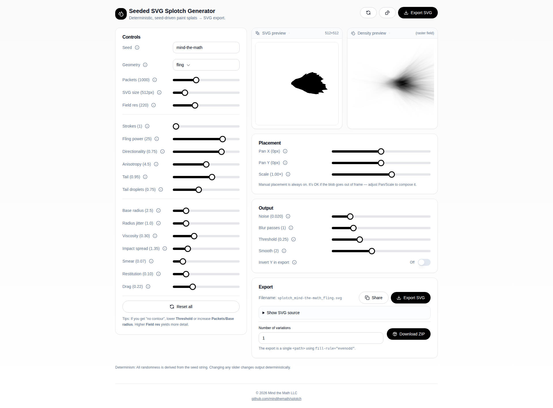
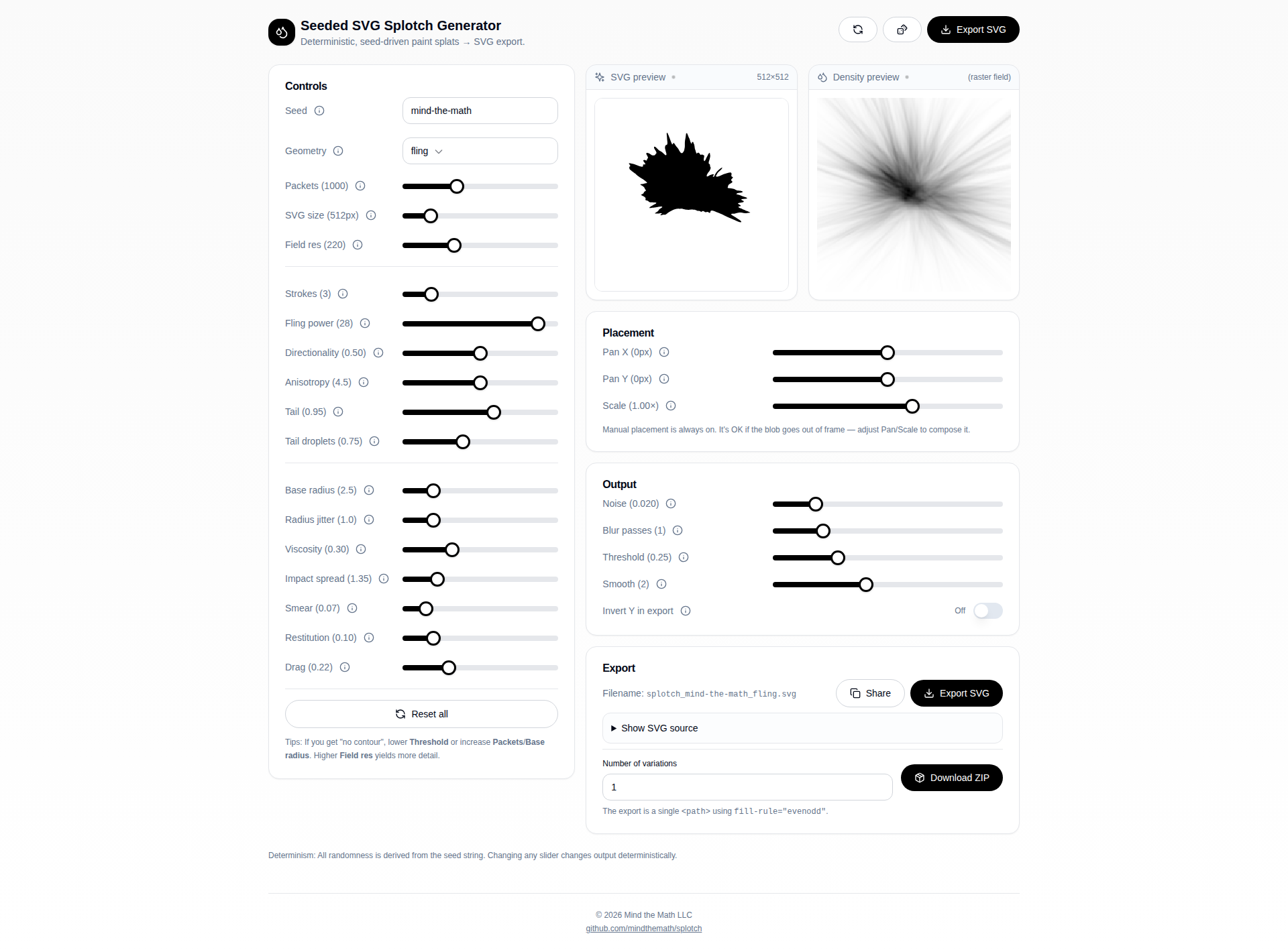
Since you have Bun installed, you can run the app with:

# Install dependencies (if you haven't already)
bun install
# Start the development server
bun run dev

The app will be available at http://localhost:5173 (or the port shown in the terminal).

Sharing Configurations

The app supports sharing complete configurations via URL parameters. All slider values and settings (except export-specific options like filename and variations count) are encoded in the URL.

Using the Share Button

Click the Share button (with the copy icon) in the Export section to copy a URL containing all current settings. When someone opens that URL, the app will automatically restore all parameters.

URL Parameter Format

Parameters use short names to keep URLs manageable. All parameters are included in the URL (defaults are not omitted to ensure compatibility if defaults change).

Parameter Name Mapping

Short Name(s)	Full Name	Description
`s`, `seed`	`seed`	Deterministic seed string
`g`, `geom`, `geometry`	`geometry`	Geometry mode: `circle`, `line`, `spray`, or `fling`
`sz`	`svgSize`	SVG export size in pixels
`fs`	`fieldSize`	Internal simulation grid resolution
`p`	`packets`	Number of paint packets simulated
`br`	`baseRadius`	Typical droplet radius
`rj`	`radiusJitter`	Random variation in droplet size
`v`	`viscosity`	Paint viscosity (resists flow)
`r`	`restitution`	Bounciness / secondary rebounds
`d`	`drag`	Air resistance during flight
`is`	`impactSpread`	Distance micro-droplets travel on impact
`sm`	`smear`	Radial outward smear during slide
`n`	`noise`	Randomness added to density field
`b`	`blur`	Post-blur passes on density field
`t`	`threshold`	Contour cutoff value
`smth`	`smooth`	Chaikin smoothing iterations
`sa`	`sprayAngleDeg`	Direction angle in degrees (0-360)
`smag`	`sprayMagnitude`	Strength of directional drift
`sc`	`sprayCovariance`	Anisotropy of spray cloud
`st`, `strokes`	`strokes`	Number of fling strokes
`fp`	`flingPower`	How hard paint is thrown
`dir`	`directionality`	Alignment tightness for fling
`an`	`anisotropy`	Elongation along velocity
`tl`	`tail`	Surface streaking length
`td`	`tailDroplets`	Probability of far droplets
`px`	`panX`	Horizontal pan offset (pixels)
`py`	`panY`	Vertical pan offset (pixels)
`us`	`userScale`	Scale multiplier
`iy`	`invertY`	Invert Y axis (0 or 1)

Note: When serializing to URL, the app uses the preferred short names (seed, geom, strokes) for readability, but accepts all aliases when reading from URLs.

Example URLs

# Set geometry to fling
?geom=fling
# Full configuration example
?seed=my-custom-seed&geom=fling&p=1200&fp=25&dir=0.8&an=5.2&sz=900&fs=220
# Using long names
?geometry=spray&seed=test&strokes=3&packets=1500

Programmatic Usage

You can programmatically construct URLs or modify existing ones. The app reads all URL parameters on page load and merges them with defaults, applying geometry-specific adjustments when needed.

Building for Production

bun run build

The built files will be in the dist directory.

Preview Production Build

bun run preview

How It Works: A Deep Dive into the Rendering Pipeline

This document explains the math and code behind the splotch generator. We'll start with the foundational concepts, build up the rendering pipeline, and then explore how each geometry mode creates different visual effects.

1. Deterministic Randomness

The entire system is built on deterministic randomness—given the same seed string, you'll always get the exact same output. This is crucial for reproducibility.

The Seed Functions

We use two functions working together: xmur3 (a hash function) and sfc32 (a pseudo-random number generator).

xmur3 takes a string and produces a sequence of 32-bit integers:

functionxmur3(str: string){leth=1779033703^str.length;for(leti=0;i<str.length;i++){h=Math.imul(h^str.charCodeAt(i),3432918353);h=(h<<13)|(h>>>19);}returnfunction(){h=Math.imul(h^(h>>>16),2246822507);h=Math.imul(h^(h>>>13),3266489909);h^=h>>>16;returnh>>>0;};}

This hash function scrambles the input string into seemingly random numbers. The magic constants (like 3432918353) are carefully chosen to produce good statistical properties.

sfc32 (Small Fast Chaotic) takes four seed values and produces random floats between 0 and 1:

functionsfc32(a: number,b: number,c: number,d: number){returnfunction(){a>>>=0;b>>>=0;c>>>=0;d>>>=0;lett=(a+b)|0;a=b^(b>>>9);b=(c+(c<<3))|0;c=(c<<21)|(c>>>11);d=(d+1)|0;t=(t+d)|0;c=(c+t)|0;return(t>>>0)/4294967296;};}

The >>> 0 operations ensure we're working with unsigned 32-bit integers. Dividing by 4294967296 (which is 2³²) converts to a float in [0, 1).

The RNG Interface

The makeRng function combines these to provide three useful random operations:

functionmakeRng(seed: string){constseedFn=xmur3(seed);constrand=sfc32(seedFn(),seedFn(),seedFn(),seedFn());constfloat=()=>rand();// [0, 1)constrange=(min,max)=>min+(max-min)*float();// [min, max)constnormal=()=>{/* Box-Muller transform */};// Normal distributionreturn{ float, range, normal };}

The Normal Distribution (Box-Muller Transform)

Many natural phenomena follow a normal distribution (bell curve). The Box-Muller transform converts uniform random numbers into normally distributed ones:

$$Z = \sqrt{-2 \ln(U_1)} \cdot \cos(2\pi U_2)$$

Where U₁ and U₂ are uniform random numbers in (0, 1). This gives us a value Z that follows the standard normal distribution (mean = 0, standard deviation = 1).

constnormal=()=>{letu=0,v=0;while(u===0)u=float();// Avoid ln(0)while(v===0)v=float();returnMath.sqrt(-2.0*Math.log(u))*Math.cos(2.0*Math.PI*v);};

This is essential for creating realistic, organic-looking distributions of paint droplets.

2. The Density Field

The core data structure is a 2D density field—a grid of floating-point values representing how much "paint" has accumulated at each pixel.

classField{w: number;// widthh: number;// heightdata: Float32Array;constructor(w: number,h: number){this.w=w;this.h=h;this.data=newFloat32Array(w*h);}}

Coordinate System

The field uses a flat array with row-major indexing:

$$\text{index} = y \cdot w + x$$

This means position (x, y) maps to array index y * w + x. The get and add methods handle bounds checking:

idx(x: number,y: number){returny*this.w+x;}get(x: number,y: number){x=clamp(x,0,this.w-1);y=clamp(y,0,this.h-1);returnthis.data[this.idx(x,y)];}add(x: number,y: number,v: number){if(x<0||y<0||x>=this.w||y>=this.h)return;this.data[this.idx(x,y)]+=v;}

Working vs. Display Resolution

The simulation uses a larger internal field (7× the display size) to prevent clipping:

constdisplayW=params.fieldSize;constworkingW=displayW*7;constfield=newField(workingW,workingW);

This buffer zone allows paint to spread without hitting boundaries, then gets cropped/transformed for the final output.

3. Depositing Paint: Gaussian Splats

When a paint droplet hits the surface, we don't just color a single pixel—we distribute the paint according to a Gaussian (bell curve) function.

The 2D Gaussian Function

A 2D Gaussian centered at the origin looks like:

$$G(x, y) = e^{-\frac{x^2 + y^2}{2\sigma^2}}$$

Where σ (sigma) controls the spread. At the center (0,0), G = 1. As you move away, the value falls off exponentially.

Isotropic (Circular) Deposits

The depositGaussian function creates circular paint splats:

functiondepositGaussian(field: Field,p: Vec2,radius: number,amount: number){constr=Math.max(1,Math.floor(radius));constx0=Math.floor(p.x);consty0=Math.floor(p.y);constsigma2=(radius*radius)/2;// Sets denominator to r²/2, effectively σ = r/2for(letdy=-r;dy<=r;dy++){for(letdx=-r;dx<=r;dx++){constdd=dx*dx+dy*dy;// Distance squaredconstw=Math.exp(-dd/Math.max(1e-6,sigma2));field.add(x0+dx,y0+dy,amount*w);}}}

The weight w follows:

$$w = e^{-\frac{dx^2 + dy^2}{\sigma^2}}$$

This creates a soft, circular blob of paint centered at position p.

Anisotropic (Elliptical) Deposits

For fling mode, we need elliptical deposits that stretch along the direction of motion. This requires rotating and scaling the coordinate system:

functiondepositAniso(field,p,major,minor,angle,amount){constca=Math.cos(angle);constsa=Math.sin(angle);constsMajor2=(major*major)/2;constsMinor2=(minor*minor)/2;for(letdy=-R;dy<=R;dy++){for(letdx=-R;dx<=R;dx++){// Rotate into the ellipse's coordinate systemconstxr=dx*ca+dy*sa;constyr=-dx*sa+dy*ca;// Apply different scales to each axisconste=(xr*xr)/sMajor2+(yr*yr)/sMinor2;constw=Math.exp(-e);field.add(x0+dx,y0+dy,amount*w);}}}

The math here involves:

Rotation: Transform (dx, dy) by angle θ:

$$\begin{bmatrix} x_r \\ y_r \end{bmatrix} = \begin{bmatrix} \cos\theta & \sin\theta \\ -\sin\theta & \cos\theta \end{bmatrix} \begin{bmatrix} dx \\ dy \end{bmatrix}$$

Elliptical Gaussian:

$$w = e^{-\left(\frac{x_r^2}{\sigma_{major}^2} + \frac{y_r^2}{\sigma_{minor}^2}\right)}$$

The major axis is aligned with the paint's velocity direction, creating streaky deposits.

4. The Physics Simulation

Each paint "packet" undergoes a simplified physics simulation before depositing on the surface.

State Variables

Each packet has:

Position: p = {x, y} (horizontal position)
Height: z (vertical distance from surface)
Velocity: v = {x, y} (horizontal velocity)
Vertical velocity: vz

The Simulation Loop

for(lets=0;s<steps;s++){// Apply drag (air resistance)v=mul(v,1-params.drag*dragGain*0.25*dt);vz*=1-params.drag*dragGain*0.35*dt;// Apply gravityvz-=1.4*dt;// Update positionp=add(p,mul(v,physW*0.015*dt));z+=vz*dt;// Check for impactif(z<=0){impacted=true;break;}}

Physics Concepts

Drag: Air resistance slows the packet. Each timestep, velocity is multiplied by a factor less than 1:

$$v_{new} = v_{old} \cdot (1 - \text{drag} \cdot dt)$$

Gravity: Vertical velocity decreases each step:

$$v_z \leftarrow v_z - g \cdot dt$$

Position Update: Basic kinematics:

$$p \leftarrow p + v \cdot dt$$

Surface Flow

After impact, paint continues to move along the surface. A flow field simulates this:

functionsurfaceFlow(p: Vec2): Vec2{constu=(p.x-center.x)/(physW*0.5);constv=(p.y-center.y)/(physW*0.5);constradial=norm({x: u,y: v});consttang={x: -radial.y,y: radial.x};constf1=mul(flowDir,0.65);// Global flow directionconstf2=mul(tang,swirl*0.55);// Swirling motionconstf3=mul(radial,-0.25);// Inward pullreturnadd(add(f1,f2),f3);}

This creates organic, paint-like spreading with:

A dominant flow direction (randomly chosen per seed)
Swirling/circular motion
Slight inward contraction

5. Contour Extraction: Marching Squares

Once the density field is complete, we need to convert it to a vector path. Marching Squares is a classic algorithm for finding contours in 2D data.

The Algorithm

For each 2×2 cell of pixels, we look at which corners are above/below the threshold:

for(lety=0;y<h-1;y++){for(letx=0;x<w-1;x++){constv00=field.get(x,y);constv10=field.get(x+1,y);constv11=field.get(x+1,y+1);constv01=field.get(x,y+1);// Create a 4-bit index based on which corners exceed thresholdletidx=0;if(v00>=threshold)idx|=1;// bit 0if(v10>=threshold)idx|=2;// bit 1if(v11>=threshold)idx|=4;// bit 2if(v01>=threshold)idx|=8;// bit 3// idx now encodes one of 16 possible configurations}}

The 16 Cases

Each configuration tells us which edges the contour crosses. The index is a 4-bit number where each bit represents a corner:

Bit 0 (value 1): top-left (v00)
Bit 1 (value 2): top-right (v10)
Bit 2 (value 4): bottom-right (v11)
Bit 3 (value 8): bottom-left (v01)

A filled circle (●) means that corner is above the threshold.

How the Bit Pattern Maps to Edges

The contour crosses an edge when the two corners on that edge have different states (one above threshold, one below). We label the four edges as:

 e0 (top)
┌─────┐
e3 │ │ e1
│ │
└─────┘
e2 (bottom)

e0: top edge (between v00 and v10)
e1: right edge (between v10 and v11)
e2: bottom edge (between v01 and v11)
e3: left edge (between v00 and v01)

For each case, we interpolate the crossing points on the relevant edges, then connect them with line segments. The case number directly determines which edges to connect via a lookup table.

Example: Case 1 has only the top-left corner above threshold (● ○ / ○ ○). The contour must cross edges e3 (left) and e0 (top) to separate the "inside" corner from the "outside" corners. So we draw a segment connecting the interpolated points on e3 and e0.

The 16 cases are:

Row 1: Four corners (single corner above threshold)

Case 1: ● ○ Case 2: ○ ● Case 4: ○ ○ Case 8: ○ ○
○ ○ ○ ○ ● ○ ○ ●
(top-left) (top-right) (bottom-right) (bottom-left)

Row 2: Four edges (two adjacent corners above threshold)

Case 3: ● ● Case 6: ○ ● Case 12: ○ ○ Case 9: ● ○
○ ○ ○ ● ● ● ● ○
(top edge) (right edge) (bottom edge) (left edge)

Row 3: "All but" cases (three corners above threshold)

Case 14: ○ ● Case 7: ● ● Case 11: ● ● Case 13: ● ○
● ● ○ ● ● ○ ● ●
(top-left) (bottom-left) (bottom-right) (top-right)

Row 4: Special cases (empty, saddles, full)

Case 0: ○ ○ Case 5: ● ○ Case 10: ○ ● Case 15: ● ●
○ ○ ○ ● ● ○ ● ●
(empty) (saddle) (saddle) (full)

Saddle points (cases 5 and 10) are ambiguous—they have two diagonally opposite corners above threshold. We resolve this by checking the center value: if the center is above threshold, we connect the two "inside" edges; otherwise, we connect the two "outside" edges.

From Case Number to Line Segments

Once we have the case number (0-15), we use a switch statement to determine which edges to connect. The algorithm interpolates crossing points on all potentially relevant edges, then connects them based on the case:

// Interpolate crossing points on all four edgesconste0=interp(p00,p10,v00,v10);// top edgeconste1=interp(p10,p11,v10,v11);// right edgeconste2=interp(p01,p11,v01,v11);// bottom edgeconste3=interp(p00,p01,v00,v01);// left edgeswitch(idx){case1: // top-left only: connect left and topcase14: // all but top-left: same pattern (inverted)addSeg(e3,e0);break;case2: // top-right only: connect top and rightcase13: // all but top-right: same pattern (inverted)addSeg(e0,e1);break;// ... etc}

Notice that complementary cases (like 1 and 14) produce the same edge connections—this is because inverting all corners flips "inside" and "outside" but follows the same edge pattern.

For each case, we generate line segments connecting edge crossing points.

Linear Interpolation

When the contour crosses an edge, we interpolate to find the exact crossing point:

functioninterp(p1: Vec2,p2: Vec2,v1: number,v2: number){constt=(threshold-v1)/(v2-v1);return{x: lerp(p1.x,p2.x,t),y: lerp(p1.y,p2.y,t)};}

If v1 = 0.2, v2 = 0.8, and threshold = 0.5:

$$t = \frac{0.5 - 0.2}{0.8 - 0.2} = \frac{0.3}{0.6} = 0.5$$

So the contour crosses exactly halfway between the two corners.

Segment Stitching

After collecting all segments, we stitch them into closed polygons by matching endpoints:

consteps=1e-3;constkey=(p: Vec2)=>`${Math.round(p.x/eps)}:${Math.round(p.y/eps)}`;// Build adjacency mapfor(constsofsegs){segMap.get(key(s.a))!.push(s);segMap.get(key(s.b))!.push(s);}// Walk segments to form polygonsfor(consts0ofsegs){if(used.has(s0))continue;constpoly: Vec2[]=[s0.a,s0.b];// ... follow connected segments until loop closes}

6. Path Smoothing: Chaikin's Algorithm

The raw marching squares output is jagged. Chaikin's algorithm smooths it by repeatedly cutting corners.

The Algorithm

For each pair of adjacent points, create two new points at 25% and 75% along the edge:

functionchaikinSmooth(poly: Vec2[],iterations: number){for(letit=0;it<iterations;it++){constout: Vec2[]=[];for(leti=0;i<pts.length;i++){constp0=pts[i];constp1=pts[(i+1)%pts.length];constq={x: lerp(p0.x,p1.x,0.25),y: lerp(p0.y,p1.y,0.25)};constr={x: lerp(p0.x,p1.x,0.75),y: lerp(p0.y,p1.y,0.75)};out.push(q,r);}pts=out;}returnpts;}

Visually:

Before: A ●──────────────────────● B
After: A ●───● Q R ●──────────● B
(25%) (75%)

Each iteration doubles the point count and rounds corners. After 2-3 iterations, sharp corners become smooth curves.

7. Geometry Modes

Now we can explore how each geometry mode creates different distributions of paint packets.

Circle Source

The simplest mode. Packets originate from a small circular region with random velocities in all directions.

if(params.geometry==="circle"){constang=rng.range(0,Math.PI*2);// Random angleconstr=Math.abs(rng.normal())*(physW*0.06);// Distance from center (normal dist)constp=add(center,{x: Math.cos(ang)*r,y: Math.sin(ang)*r});constvdir=rot({x: 1,y: 0},rng.range(0,Math.PI*2));// Random velocity directionconstv=mul(vdir,speed);return{ p, v, vz };}

Key characteristics:

Position: Normally distributed distance from center (most packets near center)
Velocity: Uniformly random direction
Result: Symmetric, roughly circular blobs

The math:

Position uses polar coordinates with normally-distributed radius:

$$r \sim |N(0, 1)| \cdot \text{scale}$$

$$\theta \sim U(0, 2\pi)$$

$$p = \text{center} + (r\cos\theta, r\sin\theta)$$

The absolute value of the normal distribution (folded normal) ensures positive radii while keeping most packets concentrated near the center.

Line Strike

Packets are distributed along a line segment, with velocity biased in the line's direction.

if(params.geometry==="line"){constang=(params.sprayAngleDeg*Math.PI)/180;constdir={x: Math.cos(ang),y: Math.sin(ang)};constperp={x: -dir.y,y: dir.x};// Perpendicular directionconstt=rng.range(-0.5,0.5);// Position along lineconstlineLen=physW*(0.05+params.sprayMagnitude*0.19);constalongOffset=t*lineLen;constperpOffset=rng.normal()*(physW*0.02);// Slight spreadconstp=add(center,add(mul(dir,alongOffset),mul(perp,perpOffset)));// Velocity with directional biasconstdrift=params.sprayMagnitude*1.8;constv=add(mul(dir,drift+baseSpeed),mul(perp,rng.normal()*0.2));return{ p, v, vz };}

Key characteristics:

Position: Uniformly distributed along a line with small perpendicular jitter
Velocity: Biased along the line direction
sprayMagnitude controls both line length and velocity strength
Result: Elongated splats with directional character

The math:

The line is parameterized by t ∈ [-0.5, 0.5]:

$$p = \text{center} + t \cdot L \cdot \hat{d} + \epsilon \cdot \hat{n}$$

Where:

L = line length
d̂ = direction unit vector
n̂ = perpendicular unit vector
ε ~ N(0, σ) = small perpendicular noise

The perpendicular vector is computed by rotating 90°:

$$\hat{n} = (-d_y, d_x)$$

Spray

The most configurable mode. Creates a Gaussian cloud of packets with controllable spread and directionality.

if(params.geometry==="spray"){constang=(params.sprayAngleDeg*Math.PI)/180;constdir={x: Math.cos(ang),y: Math.sin(ang)};constperp={x: -dir.y,y: dir.x};constcov=clamp(params.sprayCovariance,0,1);// Anisotropic spread based on covarianceconstalongStd=baseStd*(1+2.2*cov);// More spread along directionconstperpStd=baseStd*(1-0.55*cov);// Less spread perpendicularconstmeanShift=params.sprayMagnitude*(physW*0.14);constalong=rng.normal()*alongStd+meanShift*(0.25+0.75*rng.float());constacross=rng.normal()*perpStd;constp=add(center,add(mul(dir,along),mul(perp,across)));// Velocity also anisotropicconstdrift=params.sprayMagnitude*2.2;constv=add(mul(dir,drift+rng.normal()*speed*(0.55+0.65*cov)),mul(perp,rng.normal()*speed*(1.05-0.7*cov)));return{ p, v, vz };}

Key parameters:

sprayAngleDeg: Direction of the spray (0-360°)
sprayMagnitude: How far forward the cloud shifts, and velocity bias strength
sprayCovariance: How stretched vs circular the distribution is

The math:

Spray uses a bivariate normal distribution with different variances along and perpendicular to the spray direction:

$$\text{along} \sim N(\mu_{shift}, \sigma_{along}^2)$$

$$\text{across} \sim N(0, \sigma_{perp}^2)$$

The covariance parameter interpolates between circular (cov=0) and elongated (cov=1):

$$\sigma_{along} = \sigma_0 \cdot (1 + 2.2 \cdot \text{cov})$$

$$\sigma_{perp} = \sigma_0 \cdot (1 - 0.55 \cdot \text{cov})$$

When covariance is high:

σ_along increases → more spread along the direction
σ_perp decreases → less spread perpendicular
Result: Elongated, comet-like distributions

Center compensation:

To keep the splotch visually centered, the origin is shifted opposite to the spray direction:

constoffsetAmount=params.sprayMagnitude*physW*0.35;center={x: workingW/2-Math.cos(ang)*offsetAmount,y: workingW/2-Math.sin(ang)*offsetAmount,};

Fling

The most complex and expressive mode. Simulates paint being flung from a brush with multiple correlated strokes.

Stroke-Based Architecture

Unlike other modes that treat each packet independently, fling groups packets into strokes:

conststrokeCount=params.geometry==="fling" ? Math.max(1,Math.floor(params.strokes)) : 1;constpacketsPerStroke=Math.max(1,Math.floor(params.packets/strokeCount));for(leti=0;i<params.packets;i++){conststrokeIdx=Math.floor(i/packetsPerStroke);// ... packets in the same stroke share characteristics}

Each stroke has a base angle derived deterministically from the seed:

constbaseAng=(xmur3(`${params.seed}::stroke::${strokeIdx}`)()/4294967296)*Math.PI*2;

Directional Concentration (von Mises-like Sampling)

The directionality parameter controls how tightly packets cluster around the stroke's main direction:

functionsampleAngle(mu: number){constk=clamp(params.directionality,0,1);if(k<1e-6)returnrng.range(0,Math.PI*2);// Uniform when k=0constsigma=lerp(1.35,0.08,k);// Narrow when k=1returnmu+rng.normal()*sigma;}

The math:

This approximates a von Mises distribution (the circular equivalent of a normal distribution):

$$\theta \sim N(\mu, \sigma^2) \quad \text{where} \quad \sigma = 1.35 - 1.27k$$

When directionality = 0: σ = 1.35 radians (≈77°), nearly uniform
When directionality = 1: σ = 0.08 radians (≈4.6°), very concentrated

Brush Origin Sampling

Packets don't all start from the same point. They're distributed across a small "brush footprint":

functionsampleBrushOrigin(dir: Vec2){constperp={x: -dir.y,y: dir.x};constbrushWidth=physW*0.1;constalong=physW*0.1;constu=rng.range(-0.5,0.5);// Position across brushconstv=rng.range(-0.5,0.5);// Position along brushreturnadd(center,add(mul(perp,u*brushWidth),mul(dir,v*along)));}

This creates a rectangular "source region" oriented along the stroke direction.

Power-Law Velocity

Fling uses a heavy-tailed distribution for velocity magnitude—occasionally generating very fast packets:

constheavy=Math.abs(rng.normal());constpower=params.flingPower*(0.75+0.65*rng.float())*(1+0.9*heavy*heavy);

The math:

The heavy factor follows a folded normal distribution. Squaring it creates heavy tails:

$$\text{power} \propto 1 + 0.9 \cdot |N(0,1)|^2$$

Since |N(0,1)|² follows a chi-squared distribution with 1 degree of freedom, this occasionally produces values much larger than the mean, creating dramatic long splatter streaks.

Anisotropic Deposits

Fling uses elliptical (anisotropic) deposits instead of circular ones:

if(params.geometry==="fling"){constmaj=coreR*lerp(1.0,2.6,clamp((aniso-1)/7,0,1))*(0.9+0.4*sp);constmin=coreR*lerp(1.0,0.65,clamp((aniso-1)/7,0,1));depositAniso(field,p,maj,min,ang,coreAmt);}

The anisotropy parameter controls the major/minor axis ratio:

anisotropy = 1: Circular deposits (major = minor)
anisotropy = 8: Highly elongated deposits (major ≈ 2.6× minor)

The angle ang aligns the ellipse with the velocity direction:

constang=Math.atan2(tangent.y,tangent.x);

Extended Tail Simulation

Fling runs more surface-sliding steps and with decay:

constslideSteps=Math.floor(lerp(12,38,clamp(params.tail,0,1.6)/1.6));for(lett=0;t<slideSteps;t++){// ... surface flow simulation ...if(params.geometry==="fling"){constdecay=Math.exp(-t/Math.max(1,slideSteps*0.65));constmaj=rr*(1.2+2.4*decay)*(0.7+0.8*sp);constmin=rr*(0.45+0.25*decay);depositAniso(field,ps,maj,min,ang,aa*decay);}}

The math:

The exponential decay creates naturalistic fading trails:

$$\text{decay}(t) = e^{-t / \tau}$$

Where τ (tau) is about 65% of the total slide steps. This means:

At t=0: decay = 1.0 (full intensity)
At t=τ: decay ≈ 0.37
At t=2τ: decay ≈ 0.14

Both the deposit amount and the ellipse elongation decrease with the decay factor, creating tapered tails.

Tail Droplets

Additional scattered droplets break off during the tail phase:

constsplatP=0.12+0.08*(1-params.viscosity)+0.1*clamp(params.tailDroplets,0,2);if(rng.float()<splatP){consta2=rng.range(0,Math.PI*2);constdist2=coreR*rng.range(0.9,5.2)*impactEnergy*(0.7+0.6*sp);constps2=add(ps,{x: Math.cos(a2)*dist2,y: Math.sin(a2)*dist2});// ... deposit small anisotropic splat at ps2 ...}

The tailDroplets parameter increases the probability and spread of these secondary droplets, creating the characteristic scattered-droplet look of real flung paint.

Summary

The rendering pipeline transforms a seed string into an SVG through these stages:

Seed → RNG: Deterministic random number generator
Geometry sampling: Create initial packet positions and velocities
Physics simulation: Ballistic flight with drag and gravity
Impact & deposition: Gaussian/anisotropic paint splats
Surface flow: Post-impact spreading and streaking
Field processing: Blur and normalization
Marching squares: Convert density field to polygons
Chaikin smoothing: Refine jagged contours
SVG generation: Export as vector path

Each geometry mode customizes step 2 (how packets are distributed) while sharing the same downstream pipeline, creating distinctly different visual results from the same physics engine.

Features

Deterministic generation based on seed strings
Multiple geometry modes: spray, fling, circle source, line strike
Real-time preview with density field visualization
SVG export with customizable size and placement
Batch export of variations as ZIP file
Extensive parameter controls for fine-tuning the splat appearance

Name		Name	Last commit message	Last commit date
.github/workflows		.github/workflows
public		public
src		src
.eslintignore		.eslintignore
.eslintrc.json		.eslintrc.json
.gitignore		.gitignore
.prettierignore		.prettierignore
.prettierrc		.prettierrc
README.md		README.md
bun.lock		bun.lock
index.html		index.html
package.json		package.json
postcss.config.js		postcss.config.js
tailwind.config.js		tailwind.config.js
tsconfig.json		tsconfig.json
vite.config.js		vite.config.js

Uh oh!

Latest commit

History

Folders and files

Repository files navigation

Seeded SVG Splotch Generator

Running the App

Sharing Configurations

Using the Share Button

URL Parameter Format

Parameter Name Mapping

Example URLs

Programmatic Usage

Building for Production

Preview Production Build

How It Works: A Deep Dive into the Rendering Pipeline

Table of Contents

1. Deterministic Randomness

The Seed Functions

The RNG Interface

The Normal Distribution (Box-Muller Transform)

2. The Density Field

Coordinate System

Working vs. Display Resolution

3. Depositing Paint: Gaussian Splats

The 2D Gaussian Function

Isotropic (Circular) Deposits

Anisotropic (Elliptical) Deposits

4. The Physics Simulation

State Variables

The Simulation Loop

Physics Concepts

Surface Flow

5. Contour Extraction: Marching Squares

The Algorithm

The 16 Cases

How the Bit Pattern Maps to Edges

From Case Number to Line Segments

Linear Interpolation

Segment Stitching

6. Path Smoothing: Chaikin's Algorithm

The Algorithm

7. Geometry Modes

Circle Source

Line Strike

Spray

Fling

Stroke-Based Architecture

Directional Concentration (von Mises-like Sampling)

Brush Origin Sampling

Power-Law Velocity

Anisotropic Deposits

Extended Tail Simulation

Tail Droplets

Summary

Features

About

Resources

Stars

Watchers

Forks

Contributors

Languages